by Thomas Simonini
An intro to Advantage Actor Critic methods: let’s play Sonic the Hedgehog!
Since the beginning of this course, we’ve studied two different reinforcement learning methods:
- Value based methods (Q-learning, Deep Q-learning): where we learn a value function that will map each state action pair to a value. Thanks to these methods, we find the best action to take for each state — the action with the biggest value. This works well when you have a finite set of actions.
- Policy based methods (REINFORCE with Policy Gradients): where we directly optimize the policy without using a value function. This is useful when the action space is continuous or stochastic. The main problem is finding a good score function to compute how good a policy is. We use total rewards of the episode.
But both of these methods have big drawbacks. That’s why, today, we’ll study a new type of Reinforcement Learning method which we can call a “hybrid method”: Actor Critic. We’ll using two neural networks:
- a Critic that measures how good the action taken is (value-based)
- an Actor that controls how our agent behaves (policy-based)
Mastering this architecture is essential to understanding state of the art algorithms such as Proximal Policy Optimization (aka PPO). PPO is based on Advantage Actor Critic.
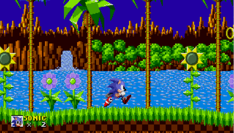
And you’ll implement an Advantage Actor Critic (A2C) agent that learns to play Sonic the Hedgehog!

The quest for a better learning model
The problem with Policy Gradients
The Policy Gradient method has a big problem. We are in a situation of Monte Carlo, waiting until the end of episode to calculate the reward. We may conclude that if we have a high reward (R(t)), all actions that we took were good, even if some were really bad.
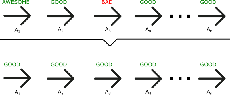
As we can see in this example, even if A3 was a bad action (led to negative rewards), all the actions will be averaged as good because the total reward was important.
As a consequence, to have an optimal policy, we need a lot of samples. This produces slow learning, because it takes a lot of time to converge.
What if, instead, we can do an update at each time step?
Introducing Actor Critic
The Actor Critic model is a better score function. Instead of waiting until the end of the episode as we do in Monte Carlo REINFORCE, we make an update at each step (TD Learning).
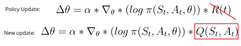
Because we do an update at each time step, we can’t use the total rewards R(t). Instead, we need to train a Critic model that approximates the value function (remember that value function calculates what is the maximum expected future reward given a state and an action). This value function replaces the reward function in policy gradient that calculates the rewards only at the end of the episode.
How Actor Critic works
Imagine you play a video game with a friend that provides you some feedback. You’re the Actor and your friend is the Critic.

At the beginning, you don’t know how to play, so you try some action randomly. The Critic observes your action and provides feedback.
Learning from this feedback, you’ll update your policy and be better at playing that game.
On the other hand, your friend (Critic) will also update their own way to provide feedback so it can be better next time.
As we can see, the idea of Actor Critic is to have two neural networks. We estimate both:


Both run in parallel.
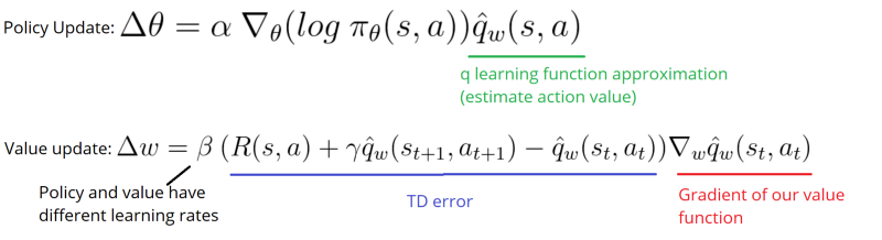
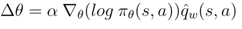
Because we have two models (Actor and Critic) that must be trained, it means that we have two set of weights (? for our action and w for our Critic) that must be optimized separately:
The Actor Critic Process
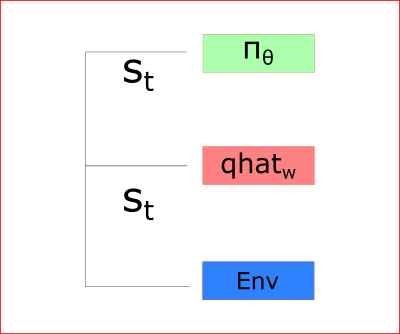
At each time-step t, we take the current state (St) from the environment and pass it as an input through our Actor and our Critic.
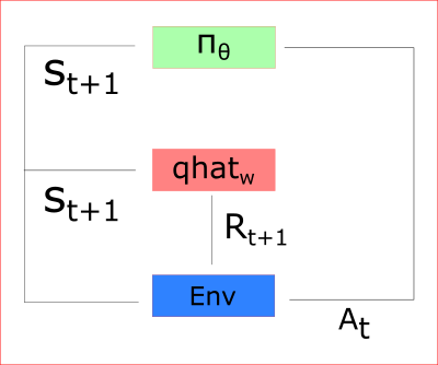
Our Policy takes the state, outputs an action (At), and receives a new state (St+1) and a reward (Rt+1).
Thanks to that:
- the Critic computes the value of taking that action at that state
- the Actor updates its policy parameters (weights) using this q value
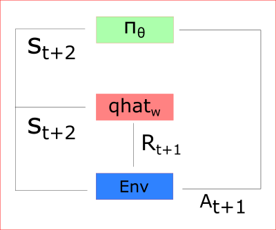
Thanks to its updated parameters, the Actor produces the next action to take at At+1 given the new state St+1. The Critic then updates its value parameters:

A2C and A3C
Introducing the Advantage function to stabilize learning
As we saw in the article about improvements in Deep Q Learning, value-based methods have high variability.
To reduce this problem, we spoke about using the advantage function instead of the value function.
The advantage function is defined like this:
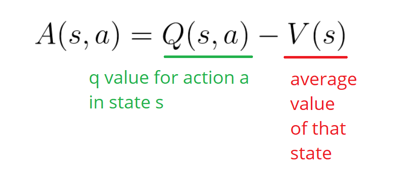
This function will tell us the improvement compared to the average the action taken at that state is. In other words, this function calculates the extra reward I get if I take this action. The extra reward is that beyond the expected value of that state.
If A(s,a) > 0: our gradient is pushed in that direction.
If A(s,a) < 0 (our action does worse than the average value of that state) our gradient is pushed in the opposite direction.
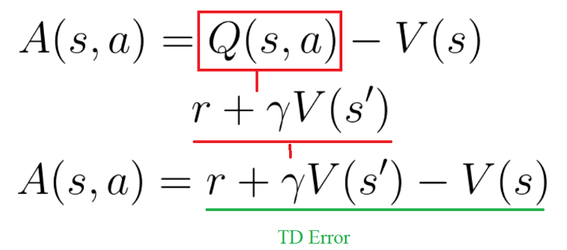
The problem of implementing this advantage function is that is requires two value functions — Q(s,a) and V(s). Fortunately, we can use the TD error as a good estimator of the advantage function.
Two different strategies: Asynchronous or Synchronous
We have two different strategies to implement an Actor Critic agent:
- A2C (aka Advantage Actor Critic)
- A3C (aka Asynchronous Advantage Actor Critic)
Because of that we will work with A2C and not A3C. If you want to see a complete implementation of A3C, check out the excellent Arthur Juliani’s A3C article and Doom implementation.
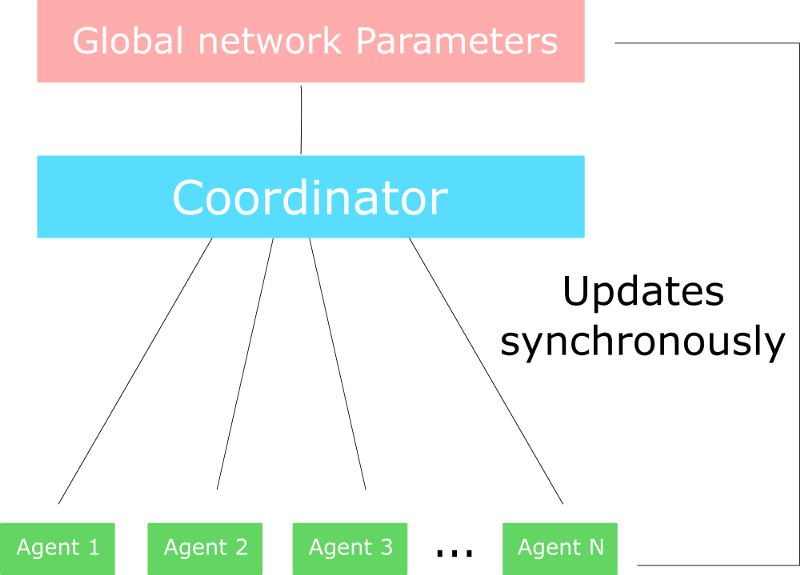
In A3C, we don’t use experience replay as this requires lot of memory. Instead, we asynchronously execute different agents in parallel on multiple instances of the environment. Each worker (copy of the network) will update the global network asynchronously.
On the other hand, the only difference in A2C is that we synchronously update the global network. We wait until all workers have finished their training and calculated their gradients to average them, to update our global network.
Choosing A2C or A3C ?
The problem of A3C is explained in this awesome article. Because of the asynchronous nature of A3C, some workers (copies of the Agent) will be playing with older version of the parameters. Thus the aggregating update will not be optimal.
That’s why A2C waits for each actor to finish their segment of experience before updating the global parameters. Then, we restart a new segment of experience with all parallel actors having the same new parameters.
As a consequence, the training will be more cohesive and faster.
Implementing an A2C agent that plays Sonic the Hedgehog
A2C in practice
In practice, as explained in this Reddit post, the synchronous nature of A2C means we don’t need different versions (different workers) of the A2C.
Each worker in A2C will have the same set of weights since, contrary to A3C, A2C updates all their workers at the same time.
In fact, we create multiple versions of environments (let say eight) and then execute them in parallel.
The process will be the following:
- Creates a vector of n environments using the multiprocessing library
- Creates a runner object that handles the different environments, executing in parallel.
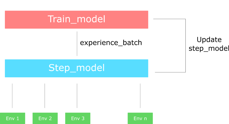
- Has two versions of the network:
- step_model: that generates experiences from environments
- train_model: that trains the experiences.
When the runner takes a step (single step model), this performs a step for each of the n environments. This outputs a batch of experience.
Then we compute the gradient all at once using train_model and our batch of experience.
Finally, we update the step model with the new weights.
Remember that computing the gradient all at once is the same thing as collecting data, calculating the gradient for each worker, and then averaging. Why? Because summing the derivatives (summing of gradients) is the same thing as taking the derivatives of the sum. But the second one is more elegant and a better way to use GPU.
A2C with Sonic the Hedgehog
So now that we understand how A2C works in general, we can implement our A2C agent playing Sonic! This video shows the behavior difference of our agent between 10 min of training (left) and 10h of training (right).
The implementation is in the GitHub repo here, and the notebook explains the implementation. I give you the saved model trained with about 10h+ on GPU.
This implementation is much complex than the former implementations. We begin to implement state of the art algorithms, so we need to be more and more efficient with our code. That’s why, in this implementation, we’ll separate the code into different objects and files.
That’s all! You’ve just created an agent that learns to play Sonic the Hedgehog. That’s awesome! We can see that with 10h of training our agent doesn’t understand the looping, for instance, so we’ll need to use a more stable architecture: PPO.
Take time to consider all the achievements you’ve made since the first chapter of this course: we went from simple text games (OpenAI taxi-v2) to complex games such as Doom and Sonic the Hedgehog using more and more powerful architectures. And that’s fantastic!
Next time we’ll learn about Proximal Policy Gradients, the architecture that won the OpenAI Retro Contest. We’ll train our agent to play Sonic the Hedgehog 2 and 3 and this time, and it will finish entire levels!
Don’t forget to implement each part of the code by yourself. It’s really important to try to modify the code I gave you. Try to add epochs, change the architecture, change the learning rate, and so forth. Experimenting is the best way to learn, so have fun!
If you liked my article, please click the ? below as many time as you liked the article so other people will see this here on Medium. And don’t forget to follow me!
This article is part of my Deep Reinforcement Learning Course with TensorFlow ?️. Check out the syllabus here.
If you have any thoughts, comments, questions, feel free to comment below or send me an email: hello [at] simoninithomas [dot] com, or tweet me @ThomasSimonini.


Deep Reinforcement Learning Course:
We’re making a video version of the Deep Reinforcement Learning Course with Tensorflow ? where we focus on the implementation part with tensorflow here.
Part 1: An introduction to Reinforcement Learning
Part 2: Diving deeper into Reinforcement Learning with Q-Learning
Part 3: An introduction to Deep Q-Learning: let’s play Doom
Part 4: An introduction to Policy Gradients with Doom and Cartpole
Part 6: Proximal Policy Optimization (PPO) with Sonic the Hedgehog 2 and 3