by Divya Godayal

An introduction to part-of-speech tagging and the Hidden Markov Model

by Sachin Malhotra and Divya Godayal

Let’s go back into the times when we had no language to communicate. The only way we had was sign language. That’s how we usually communicate with our dog at home, right? When we tell him, “We love you, Jimmy,” he responds by wagging his tail. This doesn’t mean he knows what we are actually saying. Instead, his response is simply because he understands the language of emotions and gestures more than words.

We as humans have developed an understanding of a lot of nuances of the natural language more than any animal on this planet. That is why when we say “I LOVE you, honey” vs when we say “Lets make LOVE, honey” we mean different things. Since we understand the basic difference between the two phrases, our responses are very different. It is these very intricacies in natural language understanding that we want to teach to a machine.

What this could mean is when your future robot dog hears “I love you, Jimmy”, he would know LOVE is a Verb. He would also realize that it’s an emotion that we are expressing to which he would respond in a certain way. And maybe when you are telling your partner “Lets make LOVE”, the dog would just stay out of your business ?.

This is just an example of how teaching a robot to communicate in a language known to us can make things easier.

The primary use case being highlighted in this example is how important it is to understand the difference in the usage of the word LOVE, in different contexts.

Part-of-Speech Tagging

From a very small age, we have been made accustomed to identifying part of speech tags. For example, reading a sentence and being able to identify what words act as nouns, pronouns, verbs, adverbs, and so on. All these are referred to as the part of speech tags.

Let’s look at the Wikipedia definition for them:

In corpus linguistics, part-of-speech tagging (POS tagging or PoS tagging or POST), also called grammatical tagging or word-category disambiguation, is the process of marking up a word in a text (corpus) as corresponding to a particular part of speech, based on both its definition and its context — i.e., its relationship with adjacent and related words in a phrase, sentence, or paragraph. A simplified form of this is commonly taught to school-age children, in the identification of words as nouns, verbs, adjectives, adverbs, etc.

Identifying part of speech tags is much more complicated than simply mapping words to their part of speech tags. This is because POS tagging is not something that is generic. It is quite possible for a single word to have a different part of speech tag in different sentences based on different contexts. That is why it is impossible to have a generic mapping for POS tags.

As you can see, it is not possible to manually find out different part-of-speech tags for a given corpus. New types of contexts and new words keep coming up in dictionaries in various languages, and manual POS tagging is not scalable in itself. That is why we rely on machine-based POS tagging.

Before proceeding further and looking at how part-of-speech tagging is done, we should look at why POS tagging is necessary and where it can be used.

Why Part-of-Speech tagging?

Part-of-Speech tagging in itself may not be the solution to any particular NLP problem. It is however something that is done as a pre-requisite to simplify a lot of different problems. Let us consider a few applications of POS tagging in various NLP tasks.

Text to Speech Conversion

Let us look at the following sentence:

They refuse to permit us to obtain the refuse permit.

The word refuse is being used twice in this sentence and has two different meanings here. refUSE (/rəˈfyo͞oz/)is a verb meaning “deny,” while REFuse(/ˈrefˌyo͞os/) is a noun meaning “trash” (that is, they are not homophones). Thus, we need to know which word is being used in order to pronounce the text correctly. (For this reason, text-to-speech systems usually perform POS-tagging.)

Have a look at the part-of-speech tags generated for this very sentence by the NLTK package.

>>> text = word_tokenize("They refuse to permit us to obtain the refuse permit")>>> nltk.pos_tag(text)[('They', 'PRP'), ('refuse', 'VBP'), ('to', 'TO'), ('permit', 'VB'), ('us', 'PRP'),('to', 'TO'), ('obtain', 'VB'), ('the', 'DT'), ('refuse', 'NN'), ('permit', 'NN')]

As we can see from the results provided by the NLTK package, POS tags for both refUSE and REFuse are different. Using these two different POS tags for our text to speech converter can come up with a different set of sounds.

Similarly, let us look at yet another classical application of POS tagging: word sense disambiguation.

Word Sense Disambiguation

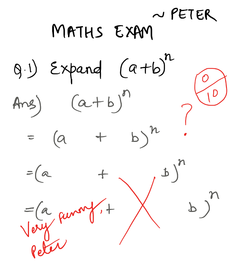
Let’s talk about this kid called Peter. Since his mother is a neurological scientist, she didn’t send him to school. His life was devoid of science and math.

One day she conducted an experiment, and made him sit for a math class. Even though he didn’t have any prior subject knowledge, Peter thought he aced his first test. His mother then took an example from the test and published it as below. (Kudos to her!)

Words often occur in different senses as different parts of speech. For example:

• She saw a bear.
• Your efforts will bear fruit.

The word bear in the above sentences has completely different senses, but more importantly one is a noun and other is a verb. Rudimentary word sense disambiguation is possible if you can tag words with their POS tags.

Word-sense disambiguation (WSD) is identifying which sense of a word (that is, which meaning) is used in a sentence, when the word has multiple meanings.

Try to think of the multiple meanings for this sentence:

Time flies like an arrow

Here are the various interpretations of the given sentence. The meaning and hence the part-of-speech might vary for each word.

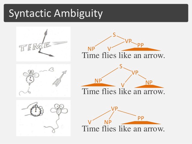
As we can clearly see, there are multiple interpretations possible for the given sentence. Different interpretations yield different kinds of part of speech tags for the words.This information, if available to us, can help us find out the exact version / interpretation of the sentence and then we can proceed from there.

The above example shows us that a single sentence can have three different POS tag sequences assigned to it that are equally likely. That means that it is very important to know what specific meaning is being conveyed by the given sentence whenever it’s appearing. This is word sense disambiguation, as we are trying to find out THE sequence.

These are just two of the numerous applications where we would require POS tagging. There are other applications as well which require POS tagging, like Question Answering, Speech Recognition, Machine Translation, and so on.

Now that we have a basic knowledge of different applications of POS tagging, let us look at how we can go about actually assigning POS tags to all the words in our corpus.

Types of POS taggers

POS-tagging algorithms fall into two distinctive groups:

• Rule-Based POS Taggers
• Stochastic POS Taggers

E. Brill’s tagger, one of the first and most widely used English POS-taggers, employs rule-based algorithms. Let us first look at a very brief overview of what rule-based tagging is all about.

Rule-Based Tagging

Automatic part of speech tagging is an area of natural language processing where statistical techniques have been more successful than rule-based methods.

Typical rule-based approaches use contextual information to assign tags to unknown or ambiguous words. Disambiguation is done by analyzing the linguistic features of the word, its preceding word, its following word, and other aspects.

For example, if the preceding word is an article, then the word in question must be a noun. This information is coded in the form of rules.

Example of a rule:

If an ambiguous/unknown word X is preceded by a determiner and followed by a noun, tag it as an adjective.

Defining a set of rules manually is an extremely cumbersome process and is not scalable at all. So we need some automatic way of doing this.

The Brill’s tagger is a rule-based tagger that goes through the training data and finds out the set of tagging rules that best define the data and minimize POS tagging errors. The most important point to note here about Brill’s tagger is that the rules are not hand-crafted, but are instead found out using the corpus provided. The only feature engineering required is a set of rule templates that the model can use to come up with new features.

Let’s move ahead now and look at Stochastic POS tagging.

Stochastic Part-of-Speech Tagging

The term ‘stochastic tagger’ can refer to any number of different approaches to the problem of POS tagging. Any model which somehow incorporates frequency or probability may be properly labelled stochastic.

The simplest stochastic taggers disambiguate words based solely on the probability that a word occurs with a particular tag. In other words, the tag encountered most frequently in the training set with the word is the one assigned to an ambiguous instance of that word. The problem with this approach is that while it may yield a valid tag for a given word, it can also yield inadmissible sequences of tags.

An alternative to the word frequency approach is to calculate the probability of a given sequence of tags occurring. This is sometimes referred to as the n-gram approach, referring to the fact that the best tag for a given word is determined by the probability that it occurs with the n previous tags. This approach makes much more sense than the one defined before, because it considers the tags for individual words based on context.

The next level of complexity that can be introduced into a stochastic tagger combines the previous two approaches, using both tag sequence probabilities and word frequency measurements. This is known as the Hidden Markov Model (HMM).

Before proceeding with what is a Hidden Markov Model, let us first look at what is a Markov Model. That will better help understand the meaning of the term Hidden in HMMs.

Markov Model

Say that there are only three kinds of weather conditions, namely

• Rainy
• Sunny
• Cloudy

Now, since our young friend we introduced above, Peter, is a small kid, he loves to play outside. He loves it when the weather is sunny, because all his friends come out to play in the sunny conditions.

He hates the rainy weather for obvious reasons.

Every day, his mother observe the weather in the morning (that is when he usually goes out to play) and like always, Peter comes up to her right after getting up and asks her to tell him what the weather is going to be like. Since she is a responsible parent, she want to answer that question as accurately as possible. But the only thing she has is a set of observations taken over multiple days as to how weather has been.

How does she make a prediction of the weather for today based on what the weather has been for the past N days?

Say you have a sequence. Something like this:

Sunny, Rainy, Cloudy, Cloudy, Sunny, Sunny, Sunny, Rainy

So, the weather for any give day can be in any of the three states.

Let’s say we decide to use a Markov Chain Model to solve this problem. Now using the data that we have, we can construct the following state diagram with the labelled probabilities.

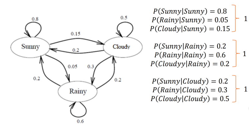
In order to compute the probability of today’s weather given N previous observations, we will use the Markovian Property.

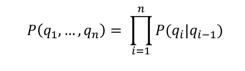
Markov Chain is essentially the simplest known Markov model, that is it obeys the Markov property.

The Markov property suggests that the distribution for a random variable in the future depends solely only on its distribution in the current state, and none of the previous states have any impact on the future states.

For a much more detailed explanation of the working of Markov chains, refer to this link.

Also, have a look at the following example just to see how probability of the current state can be computed using the formula above, taking into account the Markovian Property.

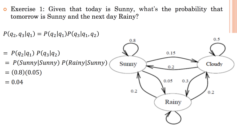
Apply the Markov property in the following example.

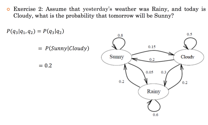
We can clearly see that as per the Markov property, the probability of tomorrow's weather being Sunny depends solely on today's weather and not on yesterday's .

Let us now proceed and see what is hidden in the Hidden Markov Models.

Hidden Markov Model

It’s the small kid Peter again, and this time he’s gonna pester his new caretaker — which is you. (Ooopsy!!)

As a caretaker, one of the most important tasks for you is to tuck Peter into bed and make sure he is sound asleep. Once you’ve tucked him in, you want to make sure he’s actually asleep and not up to some mischief.

You cannot, however, enter the room again, as that would surely wake Peter up. So all you have to decide are the noises that might come from the room. Either the room is quiet or there is noise coming from the room. These are your states.

Peter’s mother, before leaving you to this nightmare, said:

May the sound be with you :)

His mother has given you the following state diagram. The diagram has some states, observations, and probabilities.

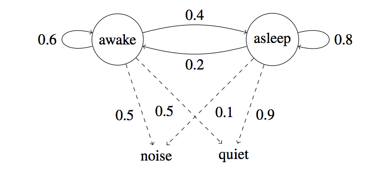
Note that there is no direct correlation between sound from the room and Peter being asleep.

There are two kinds of probabilities that we can see from the state diagram.

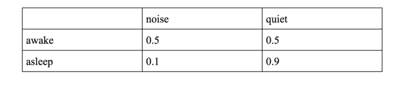
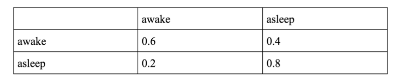
• One is the emission probabilities, which represent the probabilities of making certain observations given a particular state. For example, we have P(noise | awake) = 0.5 . This is an emission probability.
• The other ones is transition probabilities, which represent the probability of transitioning to another state given a particular state. For example, we have P(asleep | awake) = 0.4 . This is a transition probability.

The Markovian property applies in this model as well. So do not complicate things too much. Markov, your savior said:

Don’t go too much into the history…

The Markov property, as would be applicable to the example we have considered here, would be that the probability of Peter being in a state depends ONLY on the previous state.

But there is a clear flaw in the Markov property. If Peter has been awake for an hour, then the probability of him falling asleep is higher than if has been awake for just 5 minutes. So, history matters. Therefore, the Markov state machine-based model is not completely correct. It’s merely a simplification.

The Markov property, although wrong, makes this problem very tractable.

We usually observe longer stretches of the child being awake and being asleep. If Peter is awake now, the probability of him staying awake is higher than of him going to sleep. Hence, the 0.6 and 0.4 in the above diagram.P(awake | awake) = 0.6 and P(asleep | awake) = 0.4

Before actually trying to solve the problem at hand using HMMs, let’s relate this model to the task of Part of Speech Tagging.

HMMs for Part of Speech Tagging

We know that to model any problem using a Hidden Markov Model we need a set of observations and a set of possible states. The states in an HMM are hidden.

In the part of speech tagging problem, the observations are the words themselves in the given sequence.

As for the states, which are hidden, these would be the POS tags for the words.

The transition probabilities would be somewhat like P(VP | NP) that is, what is the probability of the current word having a tag of Verb Phrase given that the previous tag was a Noun Phrase.

Emission probabilities would be P(john | NP) or P(will | VP) that is, what is the probability that the word is, say, John given that the tag is a Noun Phrase.

Note that this is just an informal modeling of the problem to provide a very basic understanding of how the Part of Speech tagging problem can be modeled using an HMM.

How do we solve this?

Coming back to our problem of taking care of Peter.

Irritated are we ? ?.

Our problem here was that we have an initial state: Peter was awake when you tucked him into bed. After that, you recorded a sequence of observations, namely noise or quiet, at different time-steps. Using these set of observations and the initial state, you want to find out whether Peter would be awake or asleep after say N time steps.

We draw all possible transitions starting from the initial state. There’s an exponential number of branches that come out as we keep moving forward. So the model grows exponentially after a few time steps. Even without considering any observations. Have a look at the model expanding exponentially below.

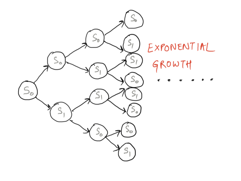
If we had a set of states, we could calculate the probability of the sequence. But we don’t have the states. All we have are a sequence of observations. This is why this model is referred to as the Hidden Markov Model — because the actual states over time are hidden.

So, caretaker, if you’ve come this far it means that you have at least a fairly good understanding of how the problem is to be structured. All that is left now is to use some algorithm / technique to actually solve the problem. For now, Congratulations on Leveling up!

In the next article of this two-part series, we will see how we can use a well defined algorithm known as the Viterbi Algorithm to decode the given sequence of observations given the model. See you there!