by Thomas Simonini
Reinforcement learning is an important type of Machine Learning where an agent learn how to behave in a environment by performing actions and seeing the results.
In recent years, we’ve seen a lot of improvements in this fascinating area of research. Examples include DeepMind and the Deep Q learning architecture in 2014, beating the champion of the game of Go with AlphaGo in 2016, OpenAI and the PPO in 2017, amongst others.
In this series of articles, we will focus on learning the different architectures used today to solve Reinforcement Learning problems. These will include Q -learning, Deep Q-learning, Policy Gradients, Actor Critic, and PPO.
In this first article, you’ll learn:
- What Reinforcement Learning is, and how rewards are the central idea
- The three approaches of Reinforcement Learning
- What the “Deep” in Deep Reinforcement Learning means
It’s really important to master these elements before diving into implementing Deep Reinforcement Learning agents.
The idea behind Reinforcement Learning is that an agent will learn from the environment by interacting with it and receiving rewards for performing actions.

Learning from interaction with the environment comes from our natural experiences. Imagine you’re a child in a living room. You see a fireplace, and you approach it.
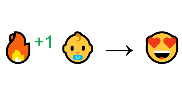
It’s warm, it’s positive, you feel good (Positive Reward +1). You understand that fire is a positive thing.
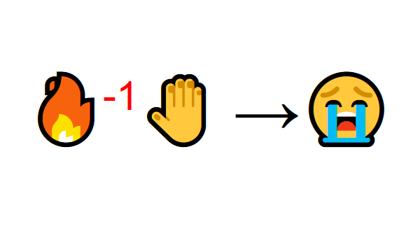
But then you try to touch the fire. Ouch! It burns your hand (Negative reward -1). You’ve just understood that fire is positive when you are a sufficient distance away, because it produces warmth. But get too close to it and you will be burned.
That’s how humans learn, through interaction. Reinforcement Learning is just a computational approach of learning from action.
The Reinforcement Learning Process
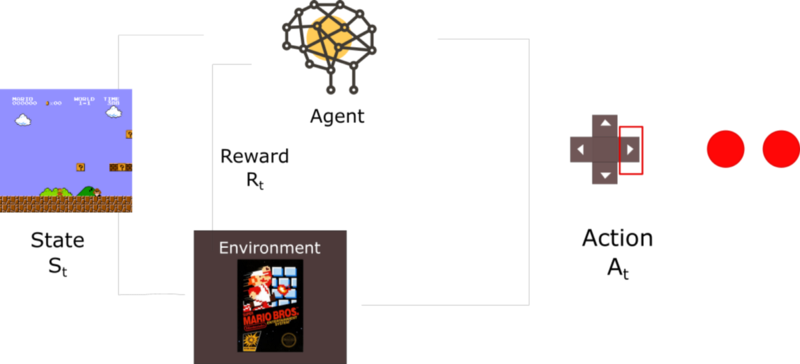
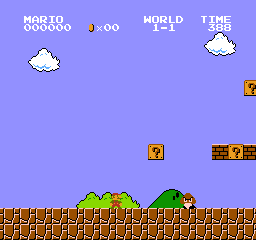
Let’s imagine an agent learning to play Super Mario Bros as a working example. The Reinforcement Learning (RL) process can be modeled as a loop that works like this:
- Our Agent receives state S0 from the Environment (In our case we receive the first frame of our game (state) from Super Mario Bros (environment))
- Based on that state S0, agent takes an action A0 (our agent will move right)
- Environment transitions to a new state S1 (new frame)
- Environment gives some reward R1 to the agent (not dead: +1)
This RL loop outputs a sequence of state, action and reward.
The goal of the agent is to maximize the expected cumulative reward.
The central idea of the Reward Hypothesis
Why is the goal of the agent to maximize the expected cumulative reward?
Well, Reinforcement Learning is based on the idea of the reward hypothesis. All goals can be described by the maximization of the expected cumulative reward.
That’s why in Reinforcement Learning, to have the best behavior, we need to maximize the expected cumulative reward.
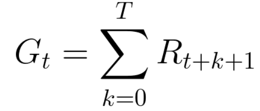
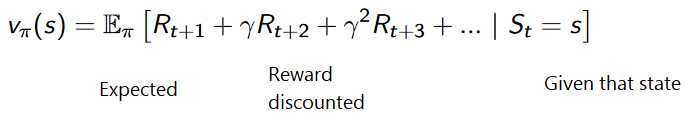
The cumulative reward at each time step t can be written as:

Which is equivalent to:
However, in reality, we can’t just add the rewards like that. The rewards that come sooner (in the beginning of the game) are more probable to happen, since they are more predictable than the long term future reward.
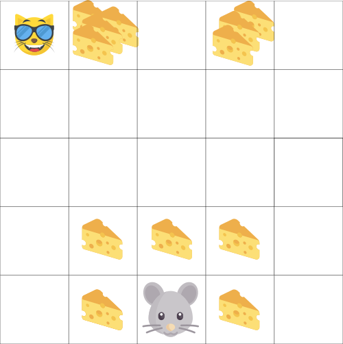
Let say your agent is this small mouse and your opponent is the cat. Your goal is to eat the maximum amount of cheese before being eaten by the cat.
As we can see in the diagram, it’s more probable to eat the cheese near us than the cheese close to the cat (the closer we are to the cat, the more dangerous it is).
As a consequence, the reward near the cat, even if it is bigger (more cheese), will be discounted. We’re not really sure we’ll be able to eat it.
To discount the rewards, we proceed like this:
We define a discount rate called gamma. It must be between 0 and 1.
- The larger the gamma, the smaller the discount. This means the learning agent cares more about the long term reward.
- On the other hand, the smaller the gamma, the bigger the discount. This means our agent cares more about the short term reward (the nearest cheese).
Our discounted cumulative expected rewards is:
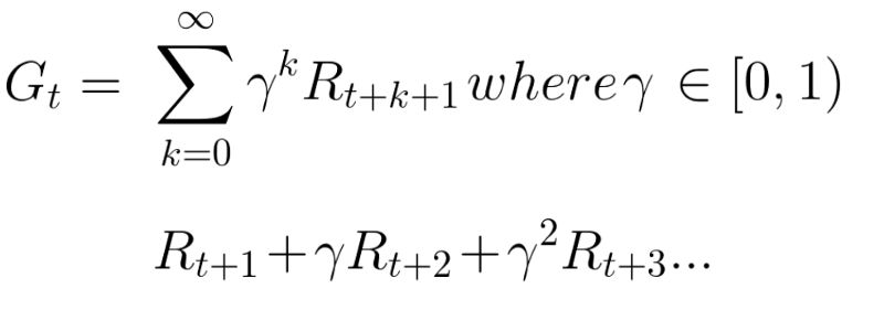
To be simple, each reward will be discounted by gamma to the exponent of the time step. As the time step increases, the cat gets closer to us, so the future reward is less and less probable to happen.
Episodic or Continuing tasks
A task is an instance of a Reinforcement Learning problem. We can have two types of tasks: episodic and continuous.
Episodic task
In this case, we have a starting point and an ending point (a terminal state). This creates an episode: a list of States, Actions, Rewards, and New States.
For instance think about Super Mario Bros, an episode begin at the launch of a new Mario and ending: when you’re killed or you’re reach the end of the level.
Continuous tasks
These are tasks that continue forever (no terminal state). In this case, the agent has to learn how to choose the best actions and simultaneously interacts with the environment.
For instance, an agent that do automated stock trading. For this task, there is no starting point and terminal state. The agent keeps running until we decide to stop him.

Monte Carlo vs TD Learning methods
We have two ways of learning:
- Collecting the rewards at the end of the episode and then calculating the maximum expected future reward: Monte Carlo Approach
- Estimate the rewards at each step: Temporal Difference Learning
Monte Carlo
When the episode ends (the agent reaches a “terminal state”), the agent looks at the total cumulative reward to see how well it did. In Monte Carlo approach, rewards are only received at the end of the game.
Then, we start a new game with the added knowledge. The agent makes better decisions with each iteration.
Let’s take an example:
If we take the maze environment:
- We always start at the same starting point.
- We terminate the episode if the cat eats us or if we move > 20 steps.
- At the end of the episode, we have a list of State, Actions, Rewards, and New States.
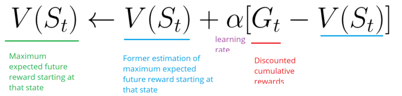
- The agent will sum the total rewards Gt (to see how well it did).
- It will then update V(st) based on the formula above.
- Then start a new game with this new knowledge.
By running more and more episodes, the agent will learn to play better and better.
Temporal Difference Learning : learning at each time step
TD Learning, on the other hand, will not wait until the end of the episode to update the maximum expected future reward estimation: it will update its value estimation V for the non-terminal states St occurring at that experience.
This method is called TD(0) or one step TD (update the value function after any individual step).
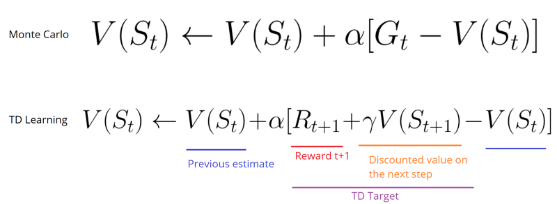
TD methods only wait until the next time step to update the value estimates. At time t+1 they immediately form a TD target using the observed reward Rt+1 and the current estimate V(St+1).
TD target is an estimation: in fact you update the previous estimate V(St) by updating it towards a one-step target.
Exploration/Exploitation trade off
Before looking at the different strategies to solve Reinforcement Learning problems, we must cover one more very important topic: the exploration/exploitation trade-off.
- Exploration is finding more information about the environment.
- Exploitation is exploiting known information to maximize the reward.
Remember, the goal of our RL agent is to maximize the expected cumulative reward. However, we can fall into a common trap.
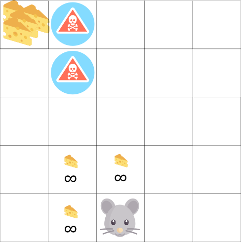
In this game, our mouse can have an infinite amount of small cheese (+1 each). But at the top of the maze there is a gigantic sum of cheese (+1000).
However, if we only focus on reward, our agent will never reach the gigantic sum of cheese. Instead, it will only exploit the nearest source of rewards, even if this source is small (exploitation).
But if our agent does a little bit of exploration, it can find the big reward.
This is what we call the exploration/exploitation trade off. We must define a rule that helps to handle this trade-off. We’ll see in future articles different ways to handle it.
Three approaches to Reinforcement Learning
Now that we defined the main elements of Reinforcement Learning, let’s move on to the three approaches to solve a Reinforcement Learning problem. These are value-based, policy-based, and model-based.
Value Based
In value-based RL, the goal is to optimize the value function V(s).
The value function is a function that tells us the maximum expected future reward the agent will get at each state.
The value of each state is the total amount of the reward an agent can expect to accumulate over the future, starting at that state.
The agent will use this value function to select which state to choose at each step. The agent takes the state with the biggest value.
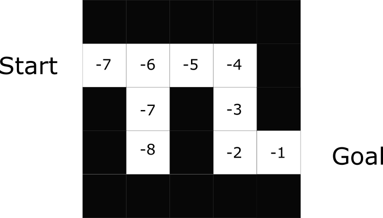
In the maze example, at each step we will take the biggest value: -7, then -6, then -5 (and so on) to attain the goal.
Policy Based
In policy-based RL, we want to directly optimize the policy function π(s) without using a value function.
The policy is what defines the agent behavior at a given time.

We learn a policy function. This lets us map each state to the best corresponding action.
We have two types of policy:
- Deterministic: a policy at a given state will always return the same action.
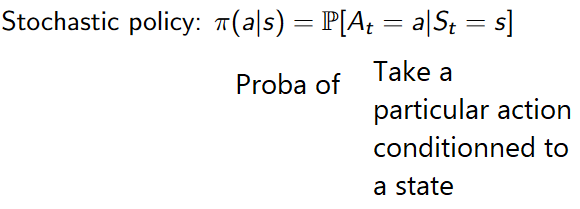
- Stochastic: output a distribution probability over actions.
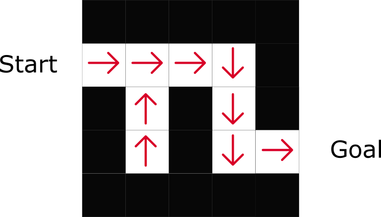
As we can see here, the policy directly indicates the best action to take for each steps.
Model Based
In model-based RL, we model the environment. This means we create a model of the behavior of the environment.
The problem is each environment will need a different model representation. That’s why we will not speak about this type of Reinforcement Learning in the upcoming articles.
Introducing Deep Reinforcement Learning
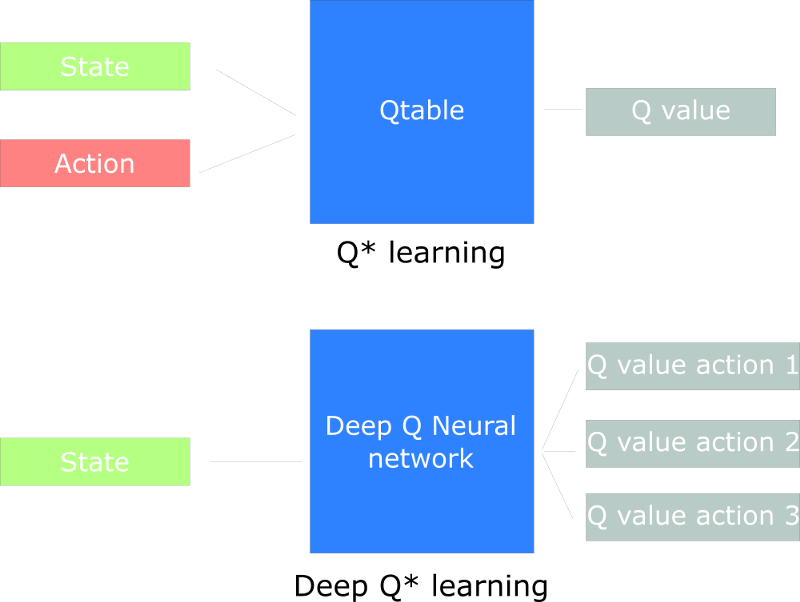
Deep Reinforcement Learning introduces deep neural networks to solve Reinforcement Learning problems — hence the name “deep.”
For instance, in the next article we’ll work on Q-Learning (classic Reinforcement Learning) and Deep Q-Learning.
You’ll see the difference is that in the first approach, we use a traditional algorithm to create a Q table that helps us find what action to take for each state.
In the second approach, we will use a Neural Network (to approximate the reward based on state: q value).
Congrats! There was a lot of information in this article. Be sure to really grasp the material before continuing. It’s important to master these elements before entering the fun part: creating AI that plays video games.
Important: this article is the first part of a free series of blog posts about Deep Reinforcement Learning. For more information and more resources, check out the syllabus.
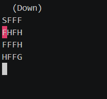
Next time we’ll work on a Q-learning agent that learns to play the Frozen Lake game.
If you liked my article, please click the ? below as many time as you liked the article so other people will see this here on Medium. And don’t forget to follow me!
If you have any thoughts, comments, questions, feel free to comment below or send me an email: hello@simoninithomas.com, or tweet me @ThomasSimonini.


Cheers!
Deep Reinforcement Learning Course:
We’re making a video version of the Deep Reinforcement Learning Course with Tensorflow ? where we focus on the implementation part with tensorflow here.
Part 1: An introduction to Reinforcement Learning
Part 2: Diving deeper into Reinforcement Learning with Q-Learning
Part 3: An introduction to Deep Q-Learning: let’s play Doom
Part 4: An introduction to Policy Gradients with Doom and Cartpole
Part 5: An intro to Advantage Actor Critic methods: let’s play Sonic the Hedgehog!
Part 6: Proximal Policy Optimization (PPO) with Sonic the Hedgehog 2 and 3