by Samay Shamdasani

How backpropagation works, and how you can use Python to build a neural network

Neural networks can be intimidating, especially for people new to machine learning. However, this tutorial will break down how exactly a neural network works and you will have a working flexible neural network by the end. Let’s get started!

Understanding the process

With approximately 100 billion neurons, the human brain processes data at speeds as fast as 268 mph! In essence, a neural network is a collection of neurons connected by synapses.

This collection is organized into three main layers: the input later, the hidden layer, and the output layer.

You can have many hidden layers, which is where the term deep learning comes into play. In an artificial neural network, there are several inputs, which are called features, which produce at least one output — which is called a label.

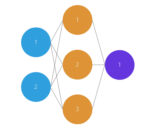
In the drawing above, the circles represent neurons while the lines represent synapses.

The role of a synapse is to take and multiply the inputs and weights.

You can think of weights as the “strength” of the connection between neurons. Weights primarily define the output of a neural network. However, they are highly flexible. After, an activation function is applied to return an output.

Here’s a brief overview of how a simple feedforward neural network works:

1. Take inputs as a matrix (2D array of numbers)
2. Multiply the inputs by a set of weights (this is done by matrix multiplication, aka taking the ‘dot product’)
3. Apply an activation function
4. Return an output
5. Error is calculated by taking the difference between the desired output from the model and the predicted output. This is a process called gradient descent, which we can use to alter the weights.
6. The weights are then adjusted, according to the error found in step 5.
7. To train, this process is repeated 1,000+ times. The more the data is trained upon, the more accurate our outputs will be.

At their core, neural networks are simple.

They just perform matrix multiplication with the input and weights, and apply an activation function.

When weights are adjusted via the gradient of loss function, the network adapts to the changes to produce more accurate outputs.

Our neural network will model a single hidden layer with three inputs and one output. In the network, we will be predicting the score of our exam based on the inputs of how many hours we studied and how many hours we slept the day before. The output is the ‘test score’.

Here’s our sample data of what we’ll be training our Neural Network on:

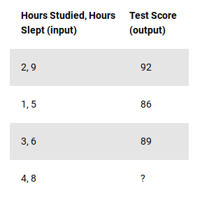
As you may have noticed, the ? in this case represents what we want our neural network to predict. In this case, we are predicting the test score of someone who studied for four hours and slept for eight hours based on their prior performance.

Forward Propagation

Let’s start coding this bad boy! Open up a new python file. You’ll want to import numpy as it will help us with certain calculations.

First, let’s import our data as numpy arrays using np.array. We'll also want to normalize our units as our inputs are in hours, but our output is a test score from 0-100. Therefore, we need to scale our data by dividing by the maximum value for each variable.

Next, let’s define a python class and write an init function where we'll specify our parameters such as the input, hidden, and output layers.

It is time for our first calculation. Remember that our synapses perform a dot product, or matrix multiplication of the input and weight. Note that weights are generated randomly and between 0 and 1.

The calculations behind our network

In the data set, our input data, X, is a 3x2 matrix. Our output data, y, is a 3x1 matrix. Each element in matrix X needs to be multiplied by a corresponding weight and then added together with all the other results for each neuron in the hidden layer. Here's how the first input data element (2 hours studying and 9 hours sleeping) would calculate an output in the network:

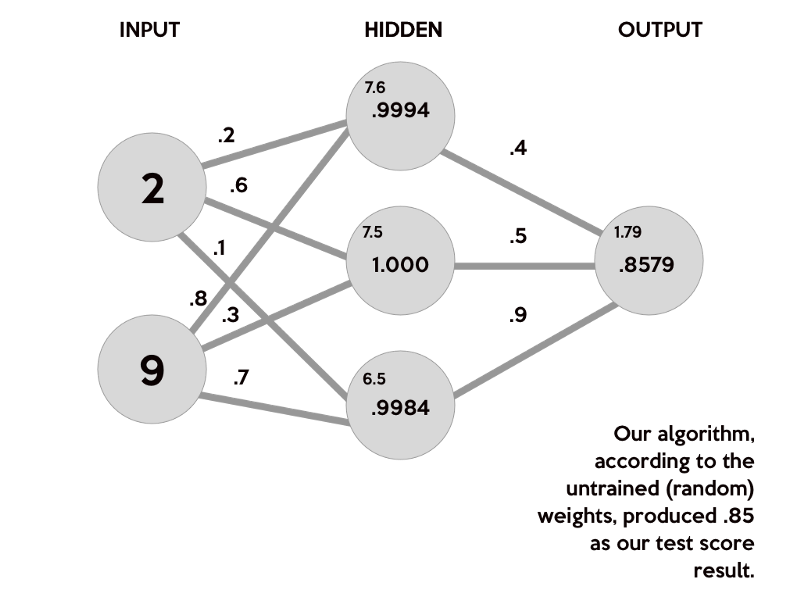
This image breaks down what our neural network actually does to produce an output. First, the products of the random generated weights (.2, .6, .1, .8, .3, .7) on each synapse and the corresponding inputs are summed to arrive as the first values of the hidden layer. These sums are in a smaller font as they are not the final values for the hidden layer.

To get the final value for the hidden layer, we need to apply the activation function.

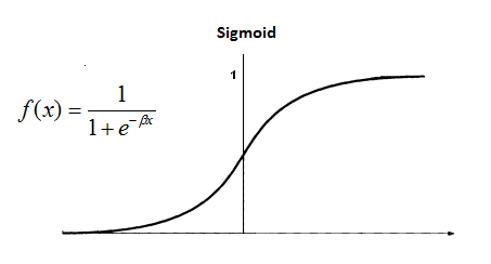
The role of an activation function is to introduce nonlinearity. An advantage of this is that the output is mapped from a range of 0 and 1, making it easier to alter weights in the future.

There are many activation functions out there, for many different use cases. In this example, we’ll stick to one of the more popular ones — the sigmoid function.

Now, we need to use matrix multiplication again, with another set of random weights, to calculate our output layer value.

Lastly, to normalize the output, we just apply the activation function again.

And, there you go! Theoretically, with those weights, out neural network will calculate .85 as our test score! However, our target was .92. Our result wasn't poor, it just isn't the best it can be. We just got a little lucky when I chose the random weights for this example.

How do we train our model to learn? Well, we’ll find out very soon. For now, let’s countinue coding our network.

If you are still confused, I highly reccomend you check out this informative video which explains the structure of a neural network with the same example.

Implementing the calculations

Now, let’s generate our weights randomly using np.random.randn(). Remember, we'll need two sets of weights. One to go from the input to the hidden layer, and the other to go from the hidden to output layer.

Once we have all the variables set up, we are ready to write our forward propagation function. Let's pass in our input, X, and in this example, we can use the variable z to simulate the activity between the input and output layers.

As explained, we need to take a dot product of the inputs and weights, apply an activation function, take another dot product of the hidden layer and second set of weights, and lastly apply a final activation function to receive our output:

Lastly, we need to define our sigmoid function:

And, there we have it! A (untrained) neural network capable of producing an output.

As you may have noticed, we need to train our network to calculate more accurate results.

Backpropagation — the “learning” of our network

Since we have a random set of weights, we need to alter them to make our inputs equal to the corresponding outputs from our data set. This is done through a method called backpropagation.

Backpropagation works by using a loss function to calculate how far the network was from the target output.

Calculating error

One way of representing the loss function is by using the mean sum squared loss function:

In this function, o is our predicted output, and y is our actual output. Now that we have the loss function, our goal is to get it as close as we can to 0. That means we will need to have close to no loss at all. As we are training our network, all we are doing is minimizing the loss.

To figure out which direction to alter the weights, we need to find the rate of change of our loss with respect to our weights. In other words, we need to use the derivative of the loss function to understand how the weights affect the input.

In this case, we will be using a partial derivative to allow us to take into account another variable.

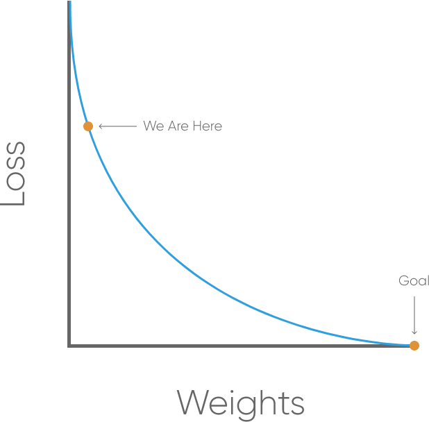
This method is known as gradient descent. By knowing which way to alter our weights, our outputs can only get more accurate.

Here’s how we will calculate the incremental change to our weights:

1. Find the margin of error of the output layer (o) by taking the difference of the predicted output and the actual output (y)
2. Apply the derivative of our sigmoid activation function to the output layer error. We call this result the delta output sum.
3. Use the delta output sum of the output layer error to figure out how much our z² (hidden) layer contributed to the output error by performing a dot product with our second weight matrix. We can call this the z² error.
4. Calculate the delta output sum for the z² layer by applying the derivative of our sigmoid activation function (just like step 2).
5. Adjust the weights for the first layer by performing a dot product of the input layer with the hidden (z²) delta output sum. For the second weight, perform a dot product of the hidden(z²) layer and the output (o) delta output sum.

Calculating the delta output sum and then applying the derivative of the sigmoid function are very important to backpropagation. The derivative of the sigmoid, also known as sigmoid prime, will give us the rate of change, or slope, of the activation function at output sum.

Let’s continue to code our Neural_Network class by adding a sigmoidPrime (derivative of sigmoid) function:

Then, we’ll want to create our backward propagation function that does everything specified in the four steps above:

We can now define our output through initiating foward propagation and intiate the backward function by calling it in the train function:

To run the network, all we have to do is to run the train function. Of course, we'll want to do this multiple, or maybe thousands, of times. So, we'll use a for loop.

Here’s the full 60 lines of awesomeness:

There you have it! A full-fledged neural network that can learn from inputs and outputs.

While we thought of our inputs as hours studying and sleeping, and our outputs as test scores, feel free to change these to whatever you like and observe how the network adapts!

After all, all the network sees are the numbers. The calculations we made, as complex as they seemed to be, all played a big role in our learning model.

If you’d like to predict an output based on our trained data, such as predicting the test score if you studied for four hours and slept for eight, check out the full tutorial here.

Demo & Source

References

Steven Miller

Welch Labs

Kabir Shah

This tutorial was originally posted on Enlight, a website that hosts a variety of tutorials and projects to learn by building! Check it out for more projects like these :)