Demystifying Gradient Descent and Backpropagation via Logistic Regression based Image…

by Sachin Malhotra

What’s all the hype about Deep Learning and what is a Neural Network anyway?

Essentially,

• you have an architecture
• with millions of parameters shared amongst thousands of neurons
• stacked up in multiple layers
• with various activation functions applied to the logits or outputs of the layers
• and normalized inputs fed with random weight initializations.
• The loss on the training batch defines the gradients for the back-propagation step through the network
• and stochastic gradient descent doing its magic to train the model and minimize the loss until convergence.

If you liked the article, do spread some love and share it as much as possible. That’s all for today folks. Hope you had a fun time reading it. ?.

You didn’t actually think I’d actually end the article amidst so much confusion about all this technical jargon, did you ? ?

If you’re someone with absolutely zero knowledge about any of this stuff and all the terms mentioned before seem Greek to you, don’t fret. Because by the end of this article, I’m sure you will be in a position to train it, test it, make it denser and hence, smarter.

Let’s get started now, shall we ?

Table of Contents

• The Age old Machine Learning Algorithm
• Data Preparation
• Say Hi to the Neuron
• Forward Propagation
• Implementation!
• Image Flattening
• Sigmoid Activation Function
• Feeding the Network ?
• Let’s Predict ?
• Let’s Go Down the Hill ?
• Enter: The loss function ?
• Minimizing the loss function ⬇️
• Does Gradient Descent Always find the Global Minima?
• Let the gradients flow ✈️
• Let’s Code! ?

The Age old Machine Learning Algorithm

Let’s start off with a very brief (well, too brief) an introduction to what one of the oldest algorithms in Machine Learning essentially does.

Take some points on a 2D graph, and draw a line that fits them as well as possible. What you have just done is generalized from a few example of pairs of input values (x) and output values (y) to a general function that can map any input value to an output value.

This is known as linear regression, and it is a wonderful technique for extrapolating a general function from some set of input-output pairs.

And here’s why having such a technique is wonderful: there are uncountable number of functions in the real world for which finding the equations is a very difficult task but collecting input-output pairs is relatively easier task to do— for instance, the function mapping an input of recorded audio of a spoken word to an output of what that spoken word is. [Source]

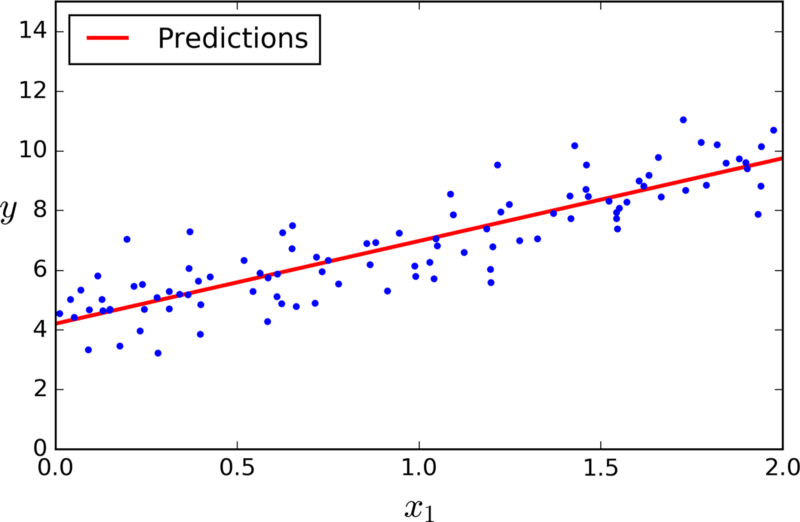
However, as we all know, we can have data that is not linearly separable. The data points might be too scattered that we cannot have a linear function to approximately map the given X values to the given Y values. A linear regression algorithm is very suitable for something like house price prediction given a set of hand crafted features. But it won’t be able to fit data that can only be approximated by a non linear function.

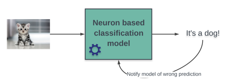
What if the problem statement is that of image classification? Say we are given an image as an input and we want our model to output if the given image is that of a cat or a dog.

How do we go about solving this problem?

Let us start off with the most basic step which is that of preparing the dataset for our model. We will explain the working of the model later on in the article.

One of the most important aspects of building any Machine Learning model is to prepare the dataset and bring it in a suitable format that the model will be able to process and draw meaningful conclusions from.

Data Preparation

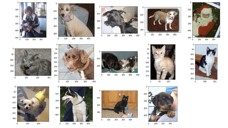
The dataset that we will be looking at in this task is the Cats v/s Dogs binary classification task available on Kaggle. Assuming that you have downloaded the dataset, let us load the dataset in memory and look at a few of the images available in the dataset.

The data is available as zip files and after unzipping, you should have two different folders. One for train and the other one for test . The test data will not be used throughout the article because we made do with the train dataset itself. The train folder has around 25000 images and we split the them into a smaller train dataset with 2000 images and another one which would server as our validation set containing 5000 images.

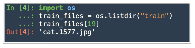
We just printed the name of a random file in the train dataset. The file names are of the type

cat.<some number>.jpg or dog.<some number>.jpg

Our model will not be able to simply process jpg files. There is some amount of work that has to be done on these images to bring the data in a certain format before our model can process it and make predictions.

Images as Matrix Representations

As discussed earlier, when training our model, we will have a certain image fed into the model and the model will give us a prediction as to whether it thinks the image is that of a cat or a dog. The model may or may not be correct and if it is not, then we have to “train” it so that it gets better at classifying cat and dog images.

A computer stores image data in the form of an M-by-N-by-3 data array that defines red, green, and blue color components for each individual pixel. So, if we look at the image data in the form of a multidimensional matrix, we have a 3D matrix with dimensions (M, N, 3) and each value will be an integer value in the range 0–255 where 0 stands for black and 1 stands for white and the remaining values make up different shades of the color components.

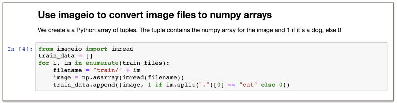
Imageio is a Python library that provides an easy interface to read and write a wide range of image data, including animated images, video, volumetric data, and scientific formats.

Numpy is a scientific computing package in Python and is one of the most fundamental libraries in Python to manipulate and work with high dimensional arrays efficiently. For a detailed primer on Numpy and how we manipulate image data, read this.

I would strongly recommend going through the Numpy tutorial mentioned above. Programming the model that we will discuss ahead is done primarily in Numpy, and a basic understanding of the operations in Numpy is extremely important.

Resizing Images

Moving on, let us look at what the numpy array for some of these images look like i.e. what is the dimensionality of some of these arrays.

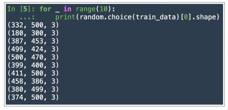
We randomly select some of the images from the list train_data that we created and we print the shape i.e. dimensions of the numpy arrays representing that image.

As we can see, the image sizes are quite varied. At the most basic level, each pixel will be an input to our image classification model and if the number of pixels are different for each image, then the model won’t be able to process them.

We need the images to be of the same size before we feed them into our model.

If you are vaguely aware of any of the Machine Learning or Deep Learning models, you must have heard of something known as the parameters of the model.

The parameters are what carry the crux of the information learnt by our models and the number of parameters for a model has to be fixed before we start training the model.

For this very reason, we cannot feed in dynamically sized images. We need to fix the size of the images and hence the number of pixels in each image so that we can define the number of inputs to our model per example and also fix the total learnable parameters for our model.

Don’t worry if you don’t have any idea about what these parameters actually are. We will get to them soon enough.

For now, the important thing is that we need all the images to be of the same size for our model to process them.

Let us see how many images have sizes more than 64-by-64 height and width.

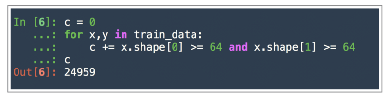
As we can clearly see, 99% of the images are have dimensions more than 64-by-64 and hence, we can downscale them to the size 64-by-64-by-3 .

This approach is just a naïve approach that I adopted to make all of the images of the same size and I felt that downscaling would not degrade the quality of the images as much as upscaling would because upscaling a very small image to a large one mostly leads to pixelated effects and would make learning for the the model tougher. Also, this dimension64-by-64-by-3 is not a magic number, just something I went with.

There would be much better approaches to data preprocessing as far as image data is concerned, but this will suffice for the current article.

Let’s move on and look at the code that would resize all of these images and also split the data into train and test sets. We split the given data using a 80/20 split, i.e. 80% of the data would be used for training our data and the remaining 20% would be used for testing out out model to see the final performance on the unseen data.

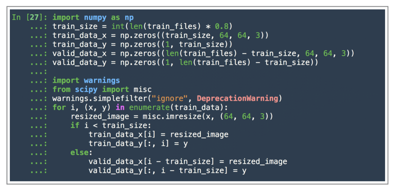
For resizing the images, we used scipy.misc.imresize method. This method will be deprecated soon, so better check out some other options for resizing images as well instead of relying on this one for your future adventures.

The reason that the inner working of the scipy.misc.imresize is not provided here is because it is not relevant to the scope of this article.

Now that we have resized our images, let us look at what our training and test data look like now, i.e. what are their final dimensions.

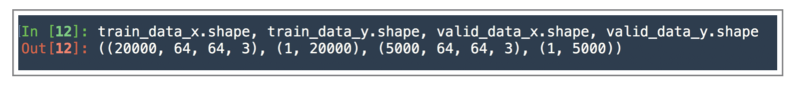
Saving the data

Now that we have processed our data and have it in the format that we need, we can finally save it into two separate files namely train.npz and valid.npz .

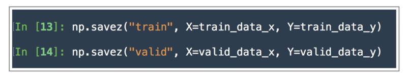
The file size of train.npz is 1.8G and that of valid.npz is 469M. These files contain the numpy arrays that we created earlier on for representing our training and test sets respectively.

Note, in this dataset we are not using any fancy deep learning architectures. We are only experimenting and showing the power of a single neuron.

As a result, we don’t have any extensive list of hyper-parameters to tune, and hence we did not split the original data into train, dev, and test. We just sufficed with a training set and a dev set (or a validation set or a test set as far as this article is concerned.) So, we use the term validation data or test data interchangeably in this article.

Note: The purpose of training data, dev or validation data, and test data are very different from one another. All three of them are extremely important

• whenever we solve any big problem with loads of data and complex architectures, and
• where we are actually concerned with the final results being on a separate held-out unseen test set.

We have no such requirements here. And hence, no separate test set.

Have a look at the Jupyter Notebook that brings all of what we discussed above together for you to see.

Say Hi to the Neuron

Now that we have preprocessed our data and we have it in a format that our binary classification model would be able to understand, allow us to introduce the core component of our model: The Neuron!

The neuron is the core computational element of our classification model. Essentially, the neuron performs something known as the forward propagation on the input data.

Let us see what this means.

Forward Propagation

Let us assume for now that our image is represented by a single real value. We will refer to this single real value as a feature representing our input image.

If you have been following along and have gone through the data preparation step, you would know that we have around 12288 features in all that represent a single image.

If you are not sure how we came at this number, don’t worry, we will come to this later.

Hint: Its 64 * 64 * 3 ?

Before we proceed, let us look at the notations that we will be following throughout this article

• small italic alphabet represents a scalar value
• small bold non-italic alphabet represents a vector i.e. either a row matrix 1-by-m or a column matrix m-by-1.
• capital italic alphabets would represents matrices of a given dimension say m-by-n .

Let x denote the single feature that represents our input image.

Now, as a first step to this process called forward propagation,

the neuron applies a linear transformation to the input feature

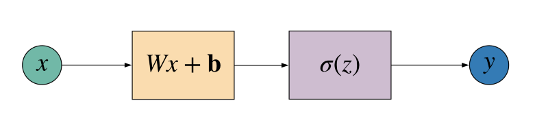
Don’t get scared by what this linear transformation means. It essentially means that we have something of the form represented by the diagram below.

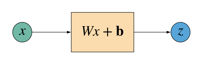
So, given the input feature x, the neuron gives us the following output:

Wx + b

Note the use of notations in the diagram and in the code section above. So, x represents a scalar value, W represents a matrix, and b represents a vector.

The matrix W is called as the weight matrix and the vector b is known as the bias vector.

Remember when we were referring to the parameters of the model earlier on? Well, the weight matrix and the bias vector would represent the parameters of our model in this scenario.

Note: that although we are referring to W as our weight “matrix” and b as our bias “vector”, in the above scenario since we only have one input feature, we only need a 1-by-1 matrix for W and a scalar value for b .

That’s all there is to the linear transformation of the input feature. We multiply it by a weight and add a bias to it to get a transformed value.

Wx + b = 94.233, What now?

That’s just a random value off the top of my head. The point I’m trying to make here is what should we do with this transformed value now?

Remember, our ultimate goal is to train a model that will be able to differentiate between a dog and a cat.

Since this is a binary classification task (just 2 classes for the model to choose from), we need to have some kind of a threshold say Θ . When the neuron generates a value above Θ , it will output one of the classes, otherwise its output would be the second class.

It is really difficult to get the range of values that a linear transformation would give. The value can be anything ranging from -inf to +inf . It all depends the range of values the input feature(s) can take and how the weight and the bias have been initialized.

So, we definitely need to fix the range of output values by the neuron.

How do we do that?

By applying what is known as an activation function to the linear output of the neuron.

The activation function will simply fix the range of output values by the neuron so that we can decide on our threshold Θ for classification output by the neuron.

Note: The activation function does a lot more than simply fixing the output values of the neuron, but again, for the scope of this article, knowing this much is more than enough.

The activation function that we will consider here is known as the Sigmoid function.

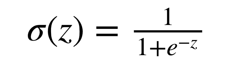
And here is the graph of the sigmoid function.

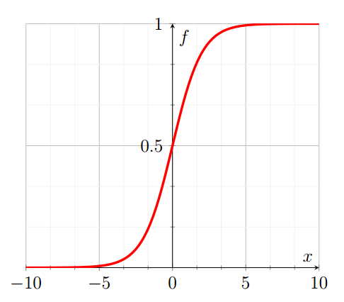
As we can see from the graph above, the sigmoid activation function applies what is known as a non linear transformation onto the input value and the range of the sigmoid function is a set of real values between [0, 1].

So, the neuron in its entirety essentially performs two operations as a part of the forward propagation process.

1. Apply a linear transformation on the input feature(s) and
2. Apply a non linear transformation (sigmoid in our case) on top of the previous output to give the final output.

But wait. You said each image has 12288 features?

We explained the calculations above assuming that the input image would be represented by a single feature value.

That is, however, not the case we are dealing with. Remember we had gone through the entire data preparation step before we started off with forward propagation and we had rescaled our images to 64-by-64-by-3?

This means that our processed image is essentially composed of 12288 pixels in all.

For our use case and the simplistic classification model that we are dealing with, we will simply consider each of the pixels as an input feature.

That means that we have 12288 input features per image for our model. Now let us see the changes this introduces into the dimensions of our model’s parameters, i.e. the weight and the bias.

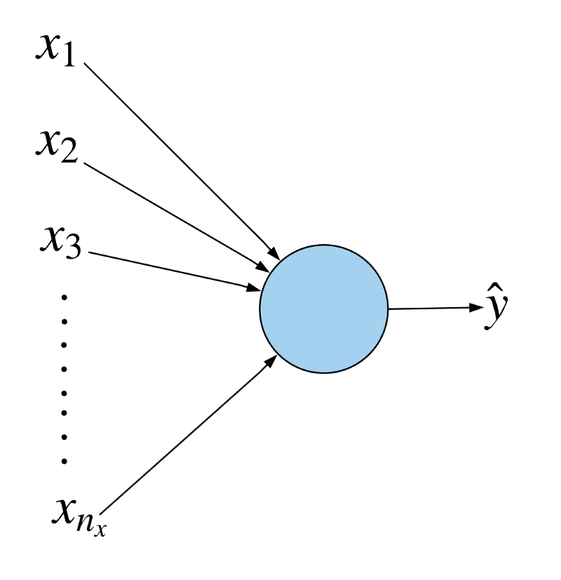
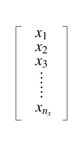
Let us represent the number of input features of our image by nx . For the images we will be considering here, the number of input features would be 12288.

So, we feed in all these input features for a given image to our neuron, it does a linear transformation on each of the features, combines the result to give a scalar value, then applies the sigmoid transformation on the value to finally give us y^ i.e. the class this image belongs to.

Note, the model simply outputs a real value between 0 and 1.

The interpretation is that if the value is > 0.5, it’s a dog/cat (whatever way you want to consider) and for all other values, its the other class.

We can either represent the input features as a column vector or a row vector . So, we can either have a vector of shape 12288-by-1) or 1-by-12288 . Let us consider the former i.e. we will have a column vector.

We will get to the coding part in the next section. It’s not a huge task to convert the 64-by-64-by-3 image pixel values to 12288-by-1 .

Earlier we had explained the forward propagation process for just a single input feature. We had a weight value for that single input feature and then we also had a bias value for it that combined and gave us the linear transformation we were looking for.

In a similar fashion, we will be needing a weight value for each of the input features. We don’t need a separate bias value for each of the features. A single value i.e. a scalar value would suffice here.

The linear transformation now becomes:

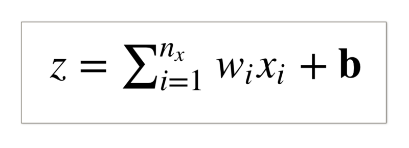
For every input feature, we multiply it with it’s corresponding weight value and then we add all these values together and finally add the bias term to get the linear transformation value.

The next step remains the same: we apply the sigmoid activation function on z and we obtain a real value between 0 and 1 (remember, that’s the range of the sigmoid function).

Implementation!

This is the fun part. ?

We will go about this in multiple steps. Just like our final Jupyter Notebook would be structured.

Retrieving the data

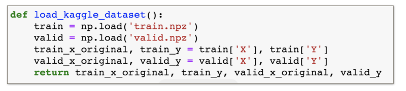
Remember we saved our data after preprocessing in two files namely train.npz and valid.npz ? We will load our data from them and return 4 different numpy arrays.

1. train_x_original represents our training set images in their original dimensions.
2. train_y contains the corresponding labels for each of the image. Just to remind you, a 1 represents a cat and a 0 represents a dog.
3. valid_x_original is the same as train_x_original except it contains the validation dataset i.e. the dataset on which we will evaluate our model’s performance.
4. valid_y are the labels for the validation set images.

Now we have our entire training and validation dataset loaded into the memory. As we discussed earlier, we want to convert all the features of the given image into either a column vector or a row vector. So, for every image, we want either a 12288-by-1 vector or a 1-by-12288 vector. Let us look at how we can do that from our original images of dimensions64-by-64-by-3 .

Image Flattening

This is a pretty straightforward task in NumPy. Given an image of dimension 64-by-64-by-3we simply want to change it’s shape to either 12288-by-1 or 1-by-12288 .

Since, we have a whole bunch of images, it would be either 12288-by-m or m-by-12288 where m represents the total number of images that we would feed our model i.e. the number of training examples.

Let us have a look at the code for this transformation.

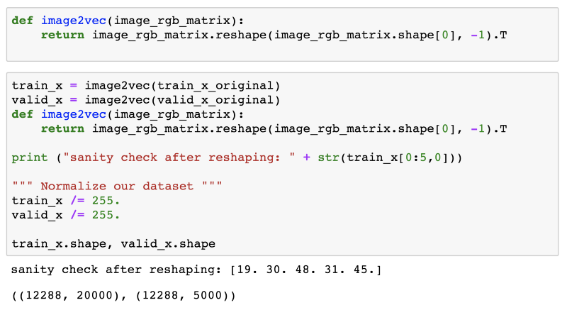
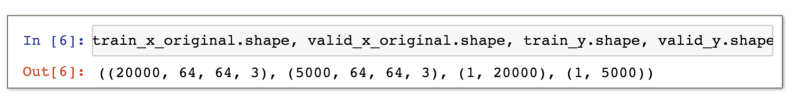
So we defined a function called as image2vec which essentially takes in our entire dataset in its original dimension i.e. 20000-by-64-by-64-by-3 for the training set and 5000-by-64-by-64-by-3 for the validation set and returns the flattened matrices.

Did you notice these lines of code?

# Normalize our datasettrain_x /= 255.valid_x /= 255.

Don’t worry, we will get to this in the next section when we discuss the activation function.

Coming back to our resulting matrix, its is a 2D one and the first index is now the number of features in each of our images i.e. 12288 and the second index represents the number of samples in that dataset which are 20000 in the training set and 5000 in the validation set.

You might ask why this specific way of arranging our data. Why didn’t we go for the transposed versions i.e. m-by-12288 where m represents the number of samples in a dataset.

I’d say we could have done that. There is nothing wrong with that arrangement of image features. However, you will notice the advantage of arranging our data in this way in the upcoming sections when we get to forward propagation for the entire dataset.

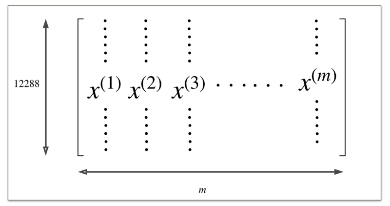
Visually, the final flattened matrix looks like this

Sigmoid Activation Function

Next step is defining our activation function. We described in the previous sections that we use a non linear activation function which for this task is the sigmoid function.

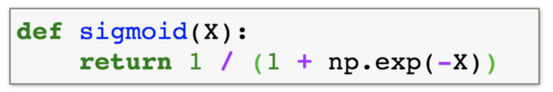
For your reference once again, here is how the sigmoid function looks like.

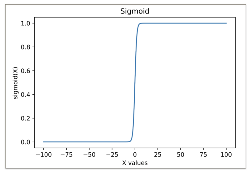
As explained before and as can be seen in the figure above,

sigmoid gives a value of 0 for very high or very low values

Hence, we need to normalize our feature values so that we don’t have too large or too small values. Let me explain this with the help of an example.

Consider the following images of cats.

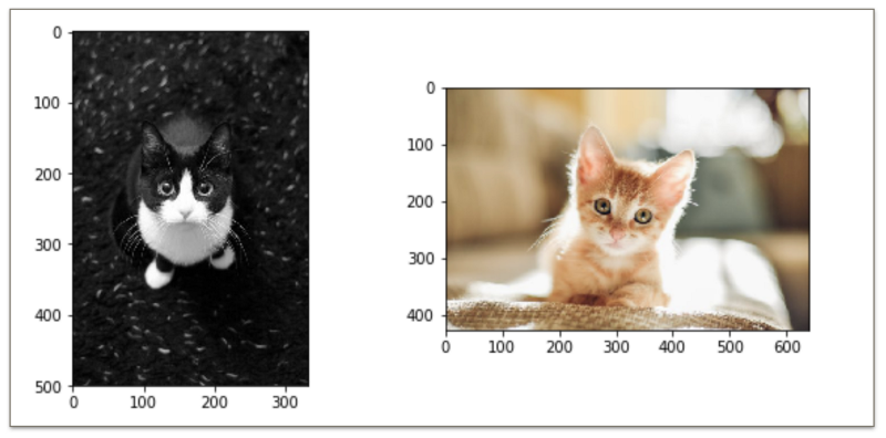
As we saw before, we have to resize our images to bring them to a fixed size. So, let us look at both these images after resizing them to 64-by-64-by-3 .

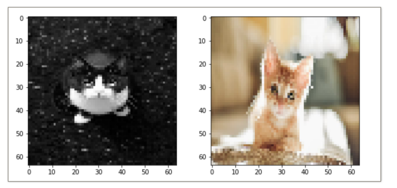
Each image is essentially is 3D matrix consisting of RGB values of different intensities and essentially they represent the colors for a given image.

The pixel values (be it for R, G or B) range from 0-255 where a 0 represents complete black and 255is for white. In between there are millions of color combinations possible.

Let’s have a look at some of the pixel values for each of these images.

[137, 109, 70, 144, 117, 74, 154, 126, 79, 160, 132, 85, 165, 137, 90, 167, 139, 92, 178, 150, 103, 186, 159, 112, 194, 170, 126, 204, 182, 143, 210, 187, 153, 212, 188, 150, 213, 185, 138, 214, 178, 121, 213, 170, 100, 212, 164, 85, 213, 158, 73, 212, 155, 65, 215, 159, 72, 215, 161, 75, 217, 162, 80, 216, 165, 82, 214, 166, 84, 212, 166, 84, 221, 187, 124, 226, 205, 160, 232, 212, 175, 236, 216, 179, 242, 220, 183, 242, 219, 177, 243, 215, 167, 243, 213, 162, 242, 213, 163, 240]

These are 100 consecutive pixel values for the colored image. What matters here is the value of each of these pixels. The values are pretty high as one would expect from a colored image as that of the brown(ish) cat shown above.

[37, 37, 37, 37, 37, 37, 29, 29, 29, 35, 35, 35, 39, 39, 39, 36, 36, 36, 38, 38, 38, 88, 88, 88, 43, 43, 43, 34, 34, 34, 33, 33, 33, 52, 52, 52, 48, 48, 48, 40, 40, 40, 33, 33, 33, 33, 33, 33, 39, 39, 39, 52, 52, 52, 36, 36, 36, 34, 34, 34, 46, 46, 46, 31, 31, 31, 34, 34, 34, 33, 33, 33, 35, 35, 35, 34, 34, 34, 26, 26, 26, 32, 32, 32, 25, 25, 25, 29, 29, 29, 23, 23, 23, 44, 44, 44, 43, 43, 43, 20]

Same set of pixel values but for the black image are the ones shown above. As we can see clearly, these values are much smaller than the values corresponding to the colored image.

The reason is straightforward in that the black and white pixel values are the ones in the vicinity of 0 and naturally, they are smaller as compared to the colored values which are in the vicinity of 255 i.e. white.

We had talked about linear transformation on the input features of the given image. For revision purposes, here is the linear transformation formula that we had used for an image with multiple features.

For the same weight matrix W and bias vector b , we will get extremely high values for the features of the colored image as compared to that of the black and white image, right ?

After this linear transformation we apply the sigmoidal activation function and we saw earlier that the sigmoid activation function gives an output of 0 for very high or very low values.

So, naturally, the sigmoid activation for the colored cat would almost always end up as 0.

How do we solve this problem one might ask?

We Normalize.

# Normalize our datasettrain_x /= 255.valid_x /= 255.

This will bring all the input features in the range [0,1] and hence all these values, be it colored images or black and white images, would have a common range. We call this process normalization of image features.

Now that we have all of our data processed and loaded in memory, the only thing that remains is our network i.e. the one powered by our single neuron. Now we will feed all these images to our model iteratively and the model will eventually learn (with some accuracy) to classify images as dogs or cats.

Just to summarize what all we we have done till now:

• Process the image dataset available to us and we converted .jpg images to numpy arrays that our model will be able to process.
• Then we loaded the two files train.npz and valid.npz in memory and we flattened the images so that we have 12288-by-1 instead of 64-by-64-by-3 images. We essentially brought all of the features for the image in a single column.
• We defined our sigmoid activation function and finally,
• We discussed why normalizing the data is a necessary step.

Now, we are ready to move on to developing our model.

Feeding the Network ?

Finally we get to the point where we are ready to feed an entire image to our network and get some predictions out of it. Let’s see how we can do that firstly for a single image and then for our entire dataset all at once.

Single Image

As discussed before, every image now has a dimension of 12288-by-1 and when we refer to the word “image”, what we really mean are the features of that image that have been flattened out and have been normalized.

For the linear transformation, we need to have a weight matrix and a bias vector. We know that the model will eventually give us a single value between 0 and 1 i.e. after applying the sigmoid activation function and hence, the bias is simply a scalar.

Essentially, we need this operation:

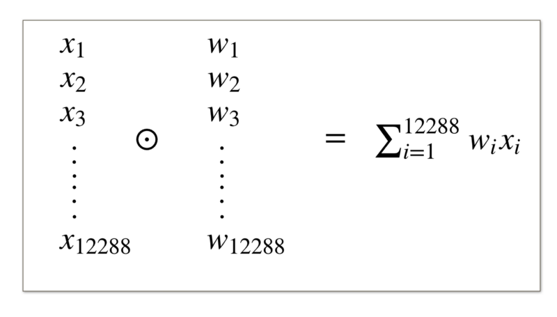
This is what is known as the Hadamard product or the element wise product of two vectors and then we do the summation of all these values.

Instead of doing this, we can use a dot product of the weight matrix and the feature vector.

The dot product of the weight matrix and the vector representing the features of the input image would give us the summation value we are looking for.

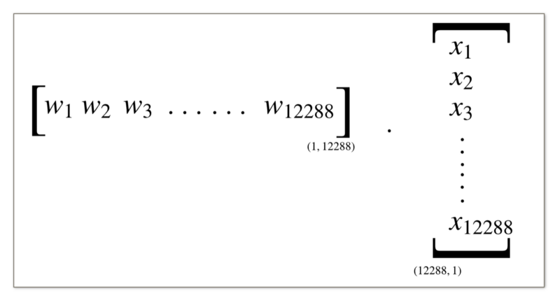
We can either define the weight matrix as a row vector and use the equation

W . x + b

or we can take the weight matrix as a column vector and then do a transpose of it for the dot product.

transpose(W) . x + b

Here, we will go with the second option. We consider the weight matrix to be of the shape 12288-by-1 for a single image. For the purpose of linear transformation, we do the transpose of the weight matrix before doing a dot product with the feature vector.

For now, just know that we want the weight values per image to be arranged in the form of a single column rather than rows. This will make the calculations a whole lot easier moving forwards.

Same goes for the input features. We want them to be arranged them in columns.

Feeding in the Entire training set

We don’t really want to process one image at a time as that would be too slow.

Ideally, we want to make a single forward pass over our model (i.e. the single neuron here) and obtain predictions for the entire training set. All in one go!

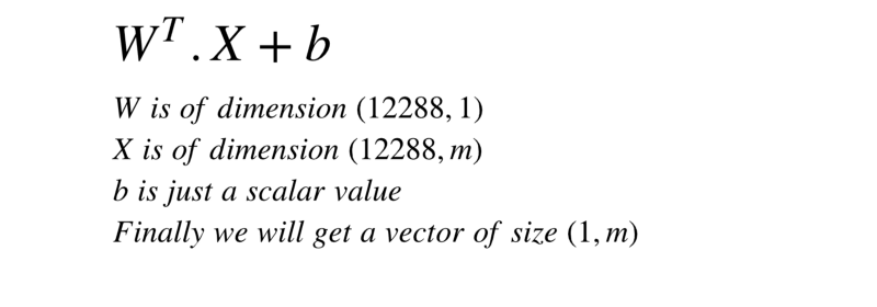
We can achieve this using the equation we looked at earlier:

transpose(W) . X + b

Note: X represents a matrix containing all of our images and x represents a single image vector.

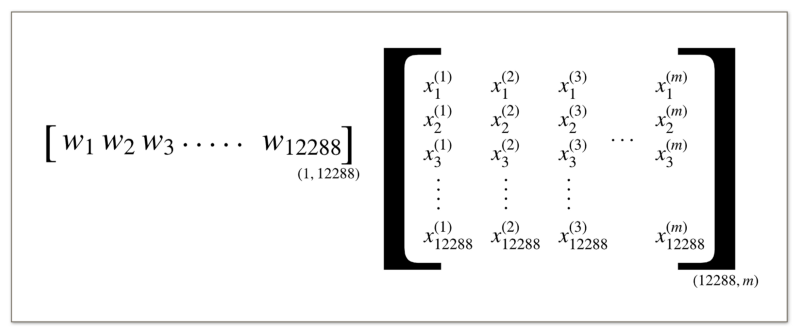
Notice the change in the notations in the equation. We were earlier using small x to denote the features of a single image.

Since we are processing our entire dataset at once, we shifted to the capital italicX notation that depicts the entire dataset and as mentioned in the figure above, it is of the dimension 12288-by-m where each image consists of 12288 features and there are m examples in all.

Let’s look at the code for this.

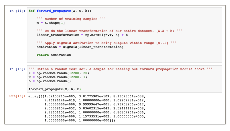
The function forward_propagate is the one doing all the heavy lifting for us. We first get the number of examples (this is not being used here, but I put it just to show that the second dimension represents number of examples).

According to the algorithm we have discussed till now, we first do a linear transformation on the input matrix X , which represents our dataset of images.

Then we apply the sigmoid activation function on the resultant matrix (vector in this case) and obtain the non linearity applied activation values from the neuron.

We initialized a random dataset here and used it to show the running and output of the forward_propagate function above.

Let’s Predict ?

Now that we have defined our neuron’s structure and the computation it performs on the image features, we are ready to make some actual classifications with our model.

But, before we do that, we need to have some sort of measure to see how well our model is actually doing on the test set.

Let’s look at the code which calculates test set accuracy of our model’s predictions. This is the core metric that we will be using throughout the remainder of our article to assess how our model is performing.

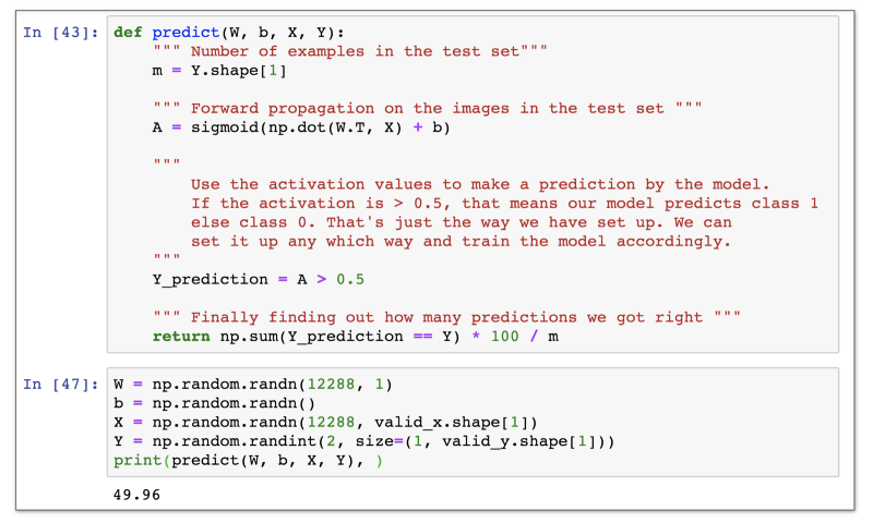
This is the code for measuring how accurate our model is in the cat vs dog classification task (test set). It turns out that an untrained model — we randomly initialized the weights and the bias values — achieves almost 50% accuracy. This is expected from a random sampler, because this is a 2 class classification task. If we pick a value from [0,1] randomly, theres a 50% probability that we will get the right value.

The question now arises, how do we improve our model?

We can improve our model by an algorithm called the Gradient Descent. Let’s move ahead and see what this algorithm is all about and how it can help us improve our model.

Let’s Go Down the Hill ?

The whole point of the gradient descent algorithm is to minimize the cost function so that our neuron-based model is able to learn.

What’s this cost function?

Our model learns as well?

I know. We need to take a step back and first go through these terms before getting to our gradient descent algorithm. So let us see exactly what is a cost function first.

Our model’s performance ?

In order to quantify how well our model is doing at the classification task, we have the metric of accuracy. Our ultimate aim is for the model’s classification accuracy to increase.

The only set of parameters controlling how accurate our model is are the weights and the bias of our neuron based model.

The reason for this is because these are the values responsible for transforming the input image features and that help us get a prediction as to whether the image is that of a dog or a cat.

We saw earlier that a random set of weights and bias value can achieve 50% classification accuracy on the test set. That means there is a lot of scope for improvement of the model.

Mathematically, we should be able to modify the weights and bias values in such a way so that the model’s accuracy becomes the best. We want those perfect set of weights and bias so that the model classifies all of the images in our test set correctly.

We have to update the model’s parameters so that it gets the highest accuracy possible on the test data of our classification task.

Consider a mathematical function like the one below:

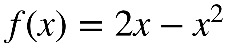
In calculus, the maxima (or minima) of any function can be found out by

• taking the first order differential of the function and equating it to 0. The point found in this way can be the point of maximum or minimum.
• Then, we substitute these values (the point we just found) into the second order differential of the function and if the value is positive i.e. > 0 then that point(s) represent the point(s) of local minima else local maxima.

If we look at the computational graph of our neuron-based model for an image consisting of just 2 features, it looks like the following:

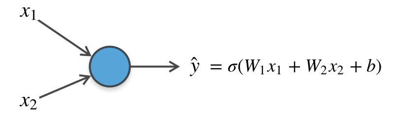
The final value we obtain is a real value between 0 and 1 and we use that to make a prediction as to whether the image is that of a dog or a cat.

Consider the following output values by the model on the same image from time to time:

0.520.560.610.670.780.800.850.890.98

By looking at these values for the same image, you would say that the model is becoming more and more confident that the image does in-fact belong to that of a cat (values > 0.5 are considered cat images in the current implementation. It’s really up-to you how you want to structure your data.)

Although the model is becoming more and more confident with its predictions, the actual prediction still remains the same i.e. a cat. For all of these values, the final prediction of the model is a cat.

This clearly highlights a big issue with using the accuracy as an optimization measure for obtaining the model’s optimal weights and biases.

We could have modeled a function centered around accuracy and maximizing it would have been our objective.

The number of images correctly classified is not a smooth function of the weights and biases in the network. For the most part, making small changes to the weights and biases won’t cause any change at all in the number of training images classified correctly.

That makes it difficult to figure out how to change the weights and biases to get improved performance. This is visible from the example that we just considered.

Although the model was getting more confident, the accuracy will never reflect this and hence, the model won’t make these sort of improvements.

What we need instead is a proxy measure that is somewhat related to the accuracy and is also a smooth function of the weights and the bias.

Enter: The loss function ?

This is a binary classification problem. That means that we can have just two classes: 0 or 1.

In a perfect world, our model would output a 0 for a dog and a 1 for a cat and in that case it would achieve 100% accuracy. Outputting a 0 for a dog or a 1 for a cat would show the model’s 100% percent confidence in its predictions. This doesn’t really happen in the real world scenario (at least not yet!).

Our untrained model will sound confused at first. It won’t be too sure about its predictions. So it might output values like 0.51, 0.49, 0.514 etc. Just because the threshold is crossed and the prediction happens to be right, doesn’t mean that our model is well trained.

From the discussion above, one thing is clear. We need to close in on the gap between the model’s output and the actual output. Lesser the gap, the better our model is at its predictions and the more confidence it shows while predicting.

This means that for a dog image, we want our model to output values as close to 0 as possible and similarly, for cat images we want our model to output values as close to 1 as possible.

This is what leads us to what is known as the loss / error / cost term for our model. The loss function essentially models the difference between our model’s prediction and the actual output. Ideally, if these two values are far apart, the loss value or the error value should be higher. Similarly, if these two values are closer, the error value should be low.

Given this sort of error function as a proxy for our model’s performance, we would like to minimize the value of this loss function.

What do you think? Is the loss function simply the distance between y_predicted and y_actual ?

|y_actual - y_predicted|

Well, we can use this specific loss function for every image and average out the loss for the entire training set to get the loss for the entire epoch. But, this is not really suitable.

The loss function below is known as the absolute difference loss function

However, it makes sense to consider this loss function for minimizing, because at the end of the day, this is the exact proxy measure that we talked about earlier that lets us in on how well our model is performing.

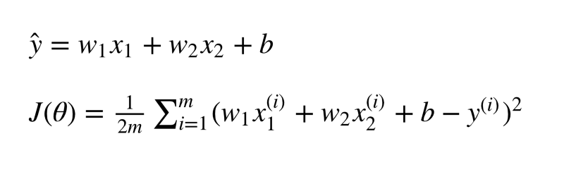
J is a common notation for the loss function and Θ represents out model’s parameters i.e. the weights and biases.

But, instead of taking this function as our loss function, we end up considering the following function.

This function is known as the squared error. We simply took the difference between the actual output y and the predicted output y^ and we squared that value (hence the name) and divided it by 2.

One of the major reasons for preferring the squared error instead of the absolute error is that the squared error is everywhere differentiable, while the absolute error is not (its derivative is undefined at 0).

To optimize the squared error, you can just set its derivative equal to 0 and solve; to optimize the absolute error often requires more complex techniques.

Additionally, the benefits of squaring include:

• Squaring always gives a positive value, so the sum will not be zero. We talk about sum here because we will add up the loss or the error values for every image in our training dataset and then we will average out to find the loss for the entire batch of training examples.
• Squaring emphasizes larger differences — a feature that turns out to be both good and bad (think of the effect outliers have).

Consider the graphs of the absolute error and squared errors respectively below.

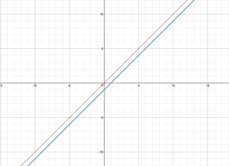
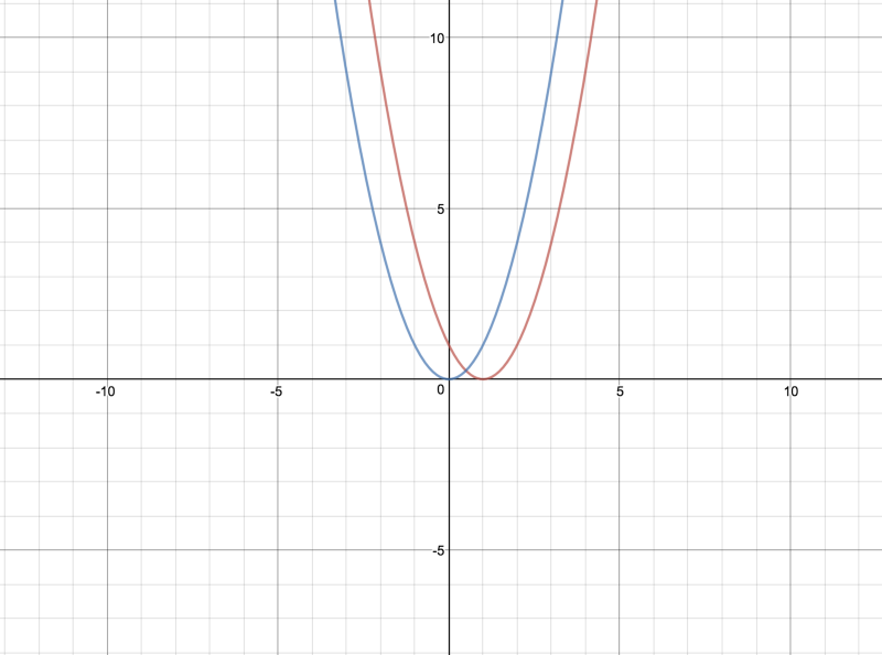
For the time being, forget the fact that we apply a sigmoid activation function to the output of the neuron before making predictions using it. Then there would be no minimum or maximum value defined for the absolute error as is clear from the graph of this function.

But, if we look at the parabolic graph for the squared function, we can see the bottom tip which is the minima of this function and this occurs at ŷ= 0 or 1 depending upon which one we are talking about. But, there’s a well defined minima for this function and hence it is easier to optimize.

That’s how I feel right now after working on this article for so long. I hope you were able to grasp all the important concepts we have discussed so far. There is still a long way to go before we wrap up.

You might wanna take a break and come back to the article, because we will start with the gradient descent algorithm now.

Ok then. Hope you are back and ready to go on!

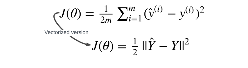
Let’s officially define the error function that we will be using here. It is known as the mean squared error and the formula is as follows.

We calculate the squared error for each image in our training set and then we find the average of these values and this represents the overall error of the model on our training set.

Minimizing the loss function ⬇️

Consider the example of a single image with just 2 features from before. Two features means that we have 2 corresponding weight values and a bias value. In all, we have 3 parameters for our model.

We want to find values for our weights and the bias that minimize the value of our loss function. Since this is a multi-variable equation, that means we would have to deal with partial derivatives of the loss function corresponding to each of our variables w1, w2 and b .

This might seem simple enough to do because we just have 3 different variables.

However, if we consider the task at hand i.e. cat v/s dog image classification using our single neuron-based model, we have 12288 weights.

Doing multivariate optimization with so many variables is computationally inefficient and is not tractable. Hence, we resort to alternatives and approximations.

Fun Fact: a typical deep neural network model has millions of weights and biases ?.

We are all set to learn about the gradient descent algorithm now.

If there’s one algorithm that’s used in almost every Machine Learning model, it’s Gradient Descent.

This is the algorithm that helps our model learn. Without the learning capability, any machine learning model is essentially as good as a random guessing model.

It’s the learning capability granted by the gradient descent algorithm that makes machine learning and deep learning models so cool.

The aim of this algorithm is to minimize the value of our loss function (surprise surprise!). And we want to do this in an efficient manner.

As discussed before, the fastest way would be to find out second order derivatives of loss function with respect to the model’s parameters. But, that is computationally expensive.

The meat of the gradient descent algorithm is the process of getting to the lowest error value. Wikipedia has a great analogy for the gradient descent algorithm:

The basic intuition behind gradient descent can be illustrated by a hypothetical scenario.

A person is stuck in the mountains and is trying to get down (i.e. trying to find the minima). There is heavy fog such that visibility is extremely low. Therefore, the path down the mountain is not visible, so they must use local information to find the minima.

They can use the method of gradient descent, which involves looking at the steepness of the hill at his current position, then proceeding in the direction with the steepest descent (i.e. downhill).

If they were trying to find the top of the mountain (i.e. the maxima), then they would proceed in the direction with the steepest ascent (i.e. uphill). Using this method, they would eventually find their way.

However, assume also that the steepness of the hill is not immediately obvious with simple observation, but rather it requires a sophisticated instrument to measure, which the person happens to have at the moment.

It takes quite some time to measure the steepness of the hill with the instrument, thus they should minimize their use of the instrument if they want to get down the mountain before sunset.

The difficulty then is choosing the frequency at which they should measure the steepness of the hill so as not to go off track.

In this analogy,

• the person represents our learning algorithm, and
• the path taken down the mountain represents the sequence of parameter updates that our model will eventually explore.
• The steepness of the hill represents the slope of the error surface at that point.
• The instrument used to measure steepness is differentiation (the slope of the error surface can be calculated by taking the derivative of the squared error function at that point). This is the approximation that we do when we apply gradient descent. We don’t really know the minimum point, but we do know the direction that will lead us to the minima (local or global) and we take a step in that direction.
• The direction the person chooses to travel in aligns with the gradient of the error surface at that point.
• The amount of time they travel before taking another measurement is the learning rate of the algorithm. This is essentially how big a step our model (or the person going downhill) decides to take each time.

For a deeper understanding and the mathematics behind the gradient descent algorithm, I would recommend going through:

Gradient Descent: All You Need to Know
Gradient Descent is THE most used learning algorithm in Machine Learning. This post shows you almost everything you…hackernoon.com

Does Gradient Descent Always find the Global Minima?

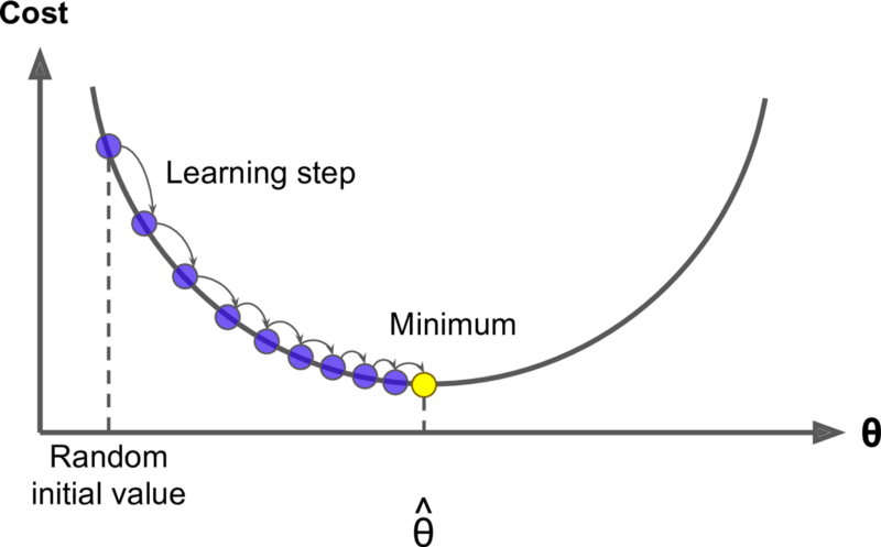
That is one of the most common figures associated with gradient descent and it shows our error function to be a smooth convex function. It also shows that the gradient descent algorithm finds the global minimum.

The loss function that we have defined is known as the mean squared loss function. The function takes in two parameters: ŷ which is the model’s prediction for a given input x and then we have y which is the actual label corresponding to that input.

Clearly, our function is a convex function with respect to the prediction ŷ.

However, if you look at the expanded equation of the loss function that we wrote a few paragraphs before, you will see that the prediction value is not something that we can control directly.

We can simply control the model’s weights and the bias value i.e. the model’s parameters and they in turn control the prediction.

Although, the mean squared loss function is convex with respect to the the prediction of the model ŷ but the convexity property that we are really interested in is with respect to the model’s parameters.

We want our loss function to be a smooth convex function of our model’s weights.

Since a typical machine learning model has millions of weights (our model has 12288 of them and it’s a single neuron), our loss function may contain multiple local minima points and the gradient descent may not necessarily find the global minima.

It all depends on the step sizes that the model takes, i.e. the learning rate, how long the model is trained for, and the amount of training data our model has.

Let the gradients flow ✈️

Ok. So by now we know that these are the two equations by which our model will learn to get better at cats and dogs image classification.

The α represents the learning rate for our gradient descent algorithm i.e. the step size for going down the hill. The term(s) next to α represent the gradients of the loss function corresponding to the weights and the bias respectively.

The question here is, how do we actually calculate these gradients?

Let us look at our computation graph for the simple model we have been working with up until now.

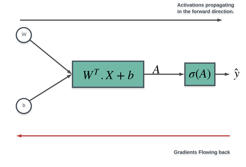
We already know how the activations flow in the forward direction. We take the input image’s features, transform them linearly, apply the sigmoid activation on the resulting value, and finally we have our activation which we then use to make a prediction.

What we will look at in this section is the flow of gradients along the red line in the diagram above by a process known as the backpropagation.

Don’t fret!

By the end of this section, you will have a clear understanding of what back-propagation is doing for us and the math behind it (at least for our specific model).

Backpropagation, is essentially the chain rule of calculus applied to computational graphs.

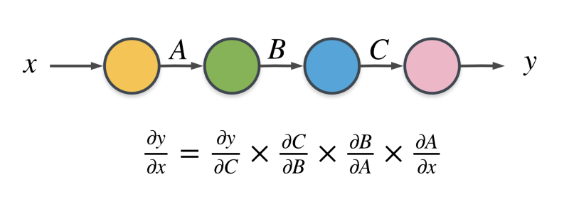
Say we wanted to find the partial derivative of the variable y with respect to x in the figure above. We can’t find that out directly because there are 3 other variables involved in the computational graph.

x --> (Some computation) --> AA --> (Some computation) --> BB --> (Some computation) --> CC --> (Some computation) --> y

So, we do this process iteratively going backwards in the computation graph.

We first find out the partial derivative of the output y with respect to the variable C . Then we use the chain rule of calculus and we determine the partial derivative with respect to the variable B and so on until we get the partial derivative we are looking for.

That’s all there is to backpropagation.

Obviously, actually finding out the derivatives in a computation graph is something that is tricky and scares most people off. However, we have a relatively simply model here at our hands and it is pretty easy to do backpropagation here. So, without further adieu, let’s get on with the mathematics of backprop on our computation graph.

Step 1: dJ/dŷ

The final equation for our loss function is:

The partial derivative of the loss function with respect to the activation of our model ŷ is:

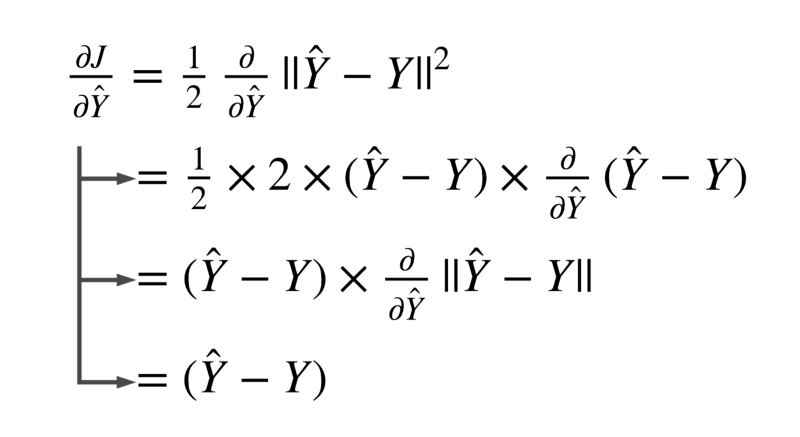
That was pretty easy!

Let’s move on one step backward and calculate our next partial derivative. This will take us one step closer to the actual gradients we want to calculate.

Step 2: dJ/dA

This is the point where we apply the chain rule we mentioned before. So, to calculate the partial derivative of the loss function with respect to the linear transformed output i.e. the output of our model before applying the sigmoid activation.:

The first part of this equation is the value we had calculated in step 1. We can simply use that here.

The essential thing to calculate here is the partial derivative of our model’s prediction with respect to the linearly transformed output, also known as the logit.

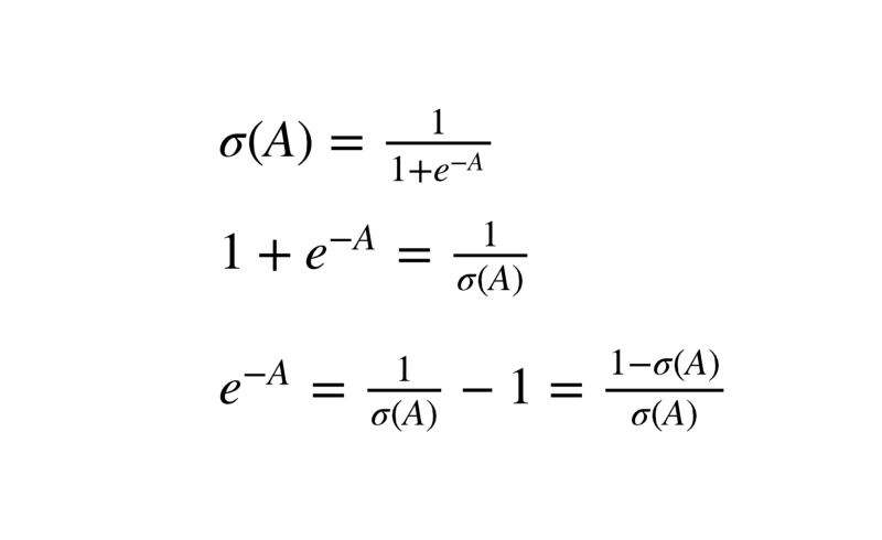
Let’s look at the equation for our model’s prediction in terms of the logit.

We have simply written the formula for the sigmoid activation function.

Derivative of our model’s final output w.r.t the logit simply means the partial derivative of the sigmoid function with respect to it’s input. Let us have a look at a derivation of the derivative ?.

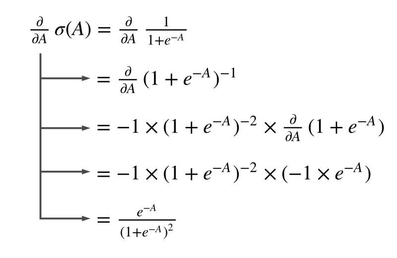
That’s quite a bit of math. But it’s just basic differential calculus here.

If you are not interested in the math and the derivation of this, you can simply look at the final values of each of these partial derivatives. You will need those to build your model from scratch.

Moving on, we can further simplify this equation.

Substituting this value in our earlier equation we get:

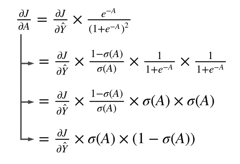
Phew! That was a lot of math, right?

But we are not done yet. There’s still one more step to go in this backpropagation algorithm.

We need to find the partial derivatives with respect to the weights and the bias yet.

Let’s move on and see how we can do that.

Step 3: dJ / dW and dJ / db

We need the partial derivative of the loss function corresponding to each of the weights. But since we are resorting to vectorization, we can find it all in one go. That is why we have been using the notation capital italic W instead of smaller w1 or w2 or any other individual weights.

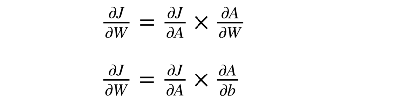
We’ll show the derivation for the weights and leave the bias portion for you to do.

Let’s Code! ?

Let us put all the math we learned in the last section into a simple function that takes in the activations vectorA and the true output labels vectorY and computes the gradients of our loss with respect to the weights and the bias.

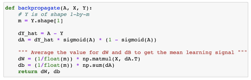
• The term dY_hat represents the partial derivative of our loss function with respect to the final output value ŷ and as shown in the previous section, that value is A — Y .
• Then we have dA which is the partial derivative with respect to the linearly transformed output, A .
• The next term is dW and we see that we have done matrix multiplication here to get that value. We divide by m to get average gradient over the entire training set. That is standard. But why have we done matrix multiplication here?

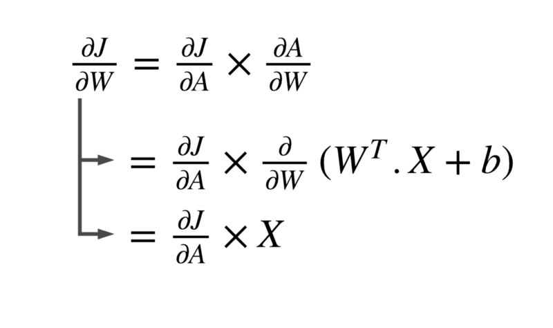
In the last figure of the previous section, we see that dJ/dW = dJ/dA * X .

Let’s take a closer look at the dimensions of the two quantities involved here. Our matrix X would be 12288-by-m where each image has 12288 features and we have m training samples.

The dimensions of the quantity dJ/dA would be the same as A and that is nothing but a single real value per training sample i.e. 1-by-m .

Also, the dimension of the quantity dJ/dW should be the same as W because ultimately, we have to subtract the gradients from the original weight values. So the two matrices must have the same dimensions.

The matrix W has a dimension of 12288-by-1 . So, we need dJ/dW to be 12288-by-1 as well. For that to happen:

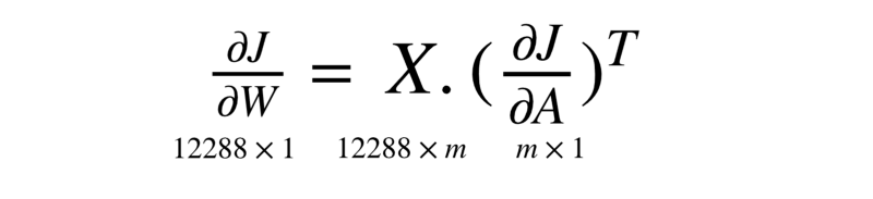
Hope this clears up why we have written the code as np.matmul(X, dZ.T) before taking the average.

Let us bring all of this together in a single comprehensive function that does the following things:

• Takes the input X and model parameters W and b and applies forward propagation on the input.
• Does backpropagation to compute the gradients.
• Applies gradient descent on the model’s parameters.
• Calculates loss on the validation dataset to measure the model’s performance and we use this to see if the model generalize well or not.

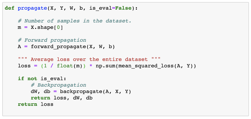
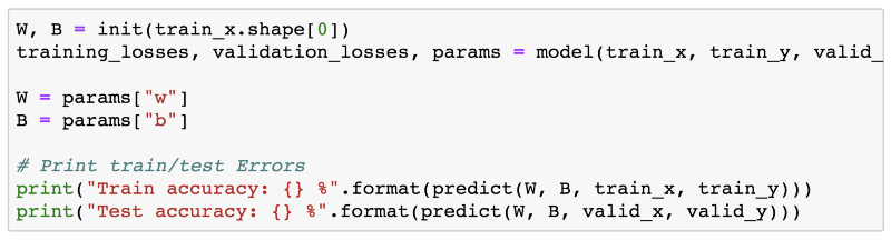
We have this combined function that does forward and backward propagation for us. So, a single call to this function and our model would have processed and learned once from our entire training set.

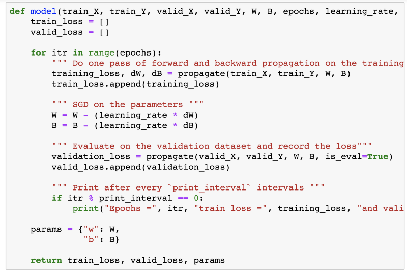
That’s the main function that essentially does the same process but multiple times.

Exposing the model multiple times to the training dataset and the model learns something new every time.

So, these iterations are known as epochs and we have this model function that for every epoch goes over the set of steps provided earlier.

Finally, we are at the stage where we can train our model and see how much a single neuron can actually learn as far as our cats vs image classification task is concerned.

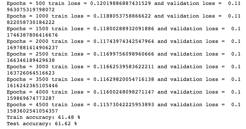
That means that on the unseen validation/test set, our model is able to predict if the image is that of a cat or a dog with 61% accuracy. That’s awesome if you ask me, because we have been able to achieve a 10% boost over a random guesser simply by using a single neuron.

Just for fun, I plotted the training and validation losses for the model’s training for all 5000 epochs.

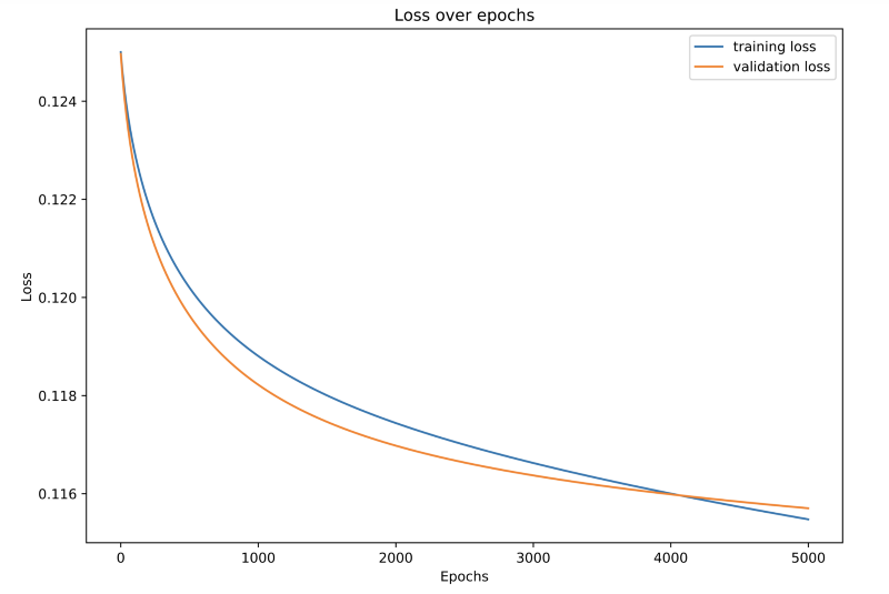
The training and validation losses decrease smoothly over time.

One final thing before I leave you to play around with the code. Let’s provide a custom image to our model, an image not a part of our dataset and see if it is able to predict correctly if the image is a cat or a dog.

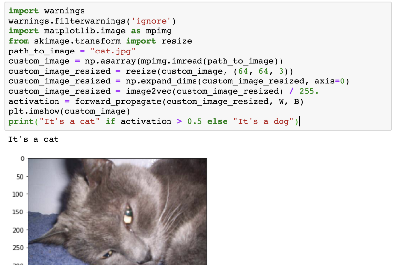
Voila! That’s correct. Indeed, that’s a cat.

For the complete code, please check out:

edorado93/Power-Of-A-Neuron
Cats vs Dogs Image Classification using Logistic Regression - edorado93/Power-Of-A-Neurongithub.com

Please recommend this post if you think this may be useful for someone! Also, feel free to point out mistakes if any in any of the calculations or the code itself. That would be much appreciated.