by Thalles Silva
Dive head first into advanced GANs: exploring self-attention and spectral norm
Lately, Generative Models are drawing a lot of attention. Much of that comes from Generative Adversarial Networks (GANs). Invented by Goodfellow et al, GANs are a framework in which two players compete with one another. The two actors, the generator G and discriminator D, are both represented by function approximators. Moreover, they play different roles in the game.
Given a training data Dt, G creates samples as an attempt to mimic the ones from the same probability distribution as Dt.
D, on the other hand, is a common binary classifier. It has two main jobs. First, it categorizes whether its received input comes from the true data distribution (Dt) or from the generator distribution. In addition, D also guides G to create more realistic samples by passing to G its gradients. In fact, taking the gradients from D is the only way G can optimize its parameters.
In this game, G takes random noise as input and generates a sample image Gsample. This sample is designed to maximize the probability of making D mistake it as coming from real training set Dt.
During training, half of the time D receives images from the training set Dt. The other half of the time, D receives images from the generator network — Gsample. D is trained to maximize the probability of assigning the correct class label to both: real images (from the training set) and fake samples (from G). In the end, the hope is that the game finds an equilibrium — the Nash equilibrium.
In this situation, G would capture the data probability distribution. And D, in turn, would not be able to distinguish between real or fake samples.
GANs have been used in a lot of different applications in the past few years. Some of them include: generating synthetic data, Image in-paining, semi-supervised learning, super-resolution, and text to image generation.
However, much of the recent work on GANs is focused on developing techniques to stabilize training. Indeed, GANs are known to be unstable during training, and very sensitive to the choice of hyper-parameters.
In this context, this piece presents an overview of two relevant techniques for improving GANs. Specifically, we aim to describe recent methods for improving the quality of G samples. To do that, we address two techniques explored in the recent paper: Self-Attention Generative Adversarial Networks.
All the code developed with the Tensorflow Eager execution API is available here.
I have a more in-depth introduction to GANs here.
Convolutional GANs
The Deep Convolutional GAN (DCGAN) was a leading step for the success of image generative GANs. DCGANs are a family of ConvNets that impose certain architectural constraints to stabilize the training of GANs.
In DCGANs, G is composed as a series of transpose convolution operations. These operations take in a random noise vector, z, and transform it by progressively increasing its spatial dimensions while decreasing its feature volume depth.
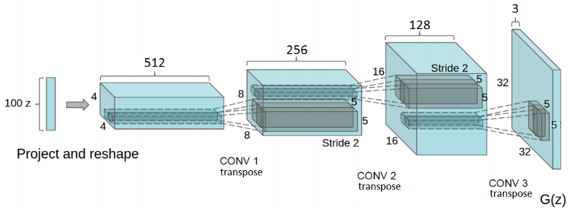
DCGAN introduced a series of architectural guidelines with the goal of stabilizing the GAN training. It advocates for the use of strided convolutions instead of pooling layers. Moreover, it uses batch normalization (BN) for both generator and discriminator nets. Finally, it uses ReLU and Tanh activations in the generator and leaky ReLUs in the discriminator.
Let’s talk about some of these guidelines.
Batch norm works by normalizing the input features of a layer to have zero mean and unit variance. BN was essential for getting Deeper models to work without falling into mode collapse. Mode collapse is the situation in which G creates samples with very low diversity. In other words, G returns the same-looking samples for different input signals. Also, BN helps to deal with problems due to poor parameter initialization.
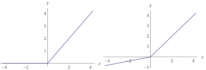
In addition, DCGAN uses Leaky ReLU activations in the discriminator net. Different from the regular ReLU function, Leaky ReLUs allow the pass of a small gradient signal for negative values. As a result, it makes the gradients from the discriminator flow stronger into the generator. Instead of passing a gradient (slope) of 0 in the back-prop pass for negative values, it passes a small negative gradient.
The architectural guidelines introduced by DCGANs are still present in the design of recent models. However, much of the work focuses on how to make the GAN training more stable.
Self-Attention GANs
Self-Attention for Generative Adversarial Networks (SAGANs) is one of these designs. Recently, attention techniques have been explored, with success, in problems like Machine Translation. Self-Attention GANs have an architecture that allows G to model long-range dependency. The key idea is to enable G to produce samples with global detailing information.
If we look at the DCGAN model, we see that regular GANs are heavily based on convolutions. These operations use a local receptive field, the convolutional kernel, to learn representations. Convolutions have very nice properties such as parameter sharing and translation invariance.
A typical Deep ConvNet learns representations in a hierarchical fashion. For a regular image classification ConvNet, simple features like edges and corners are learned in the first few layers. Yet, ConvNets are able to use these simple representations to learn more complex ones. In short, ConvNets learn representations that are expressed in terms of simpler representations. Consequently, long-range dependency might be hard to learn.
Indeed, it might only be possible for low resolution feature vectors. The problem is that, at this granularity, the amount of signal loss is such that it becomes difficult to model long-range details.
Take a look at these sample images:
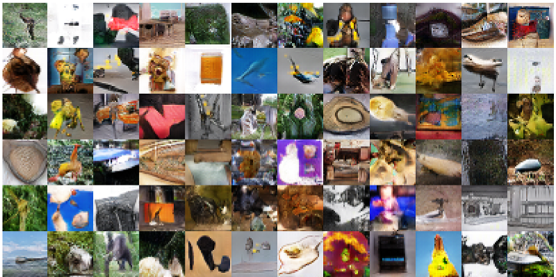
These images are from the DCGAN model trained on ImageNet. As pointed at Self-Attention GANs, most of the image content that does not exhibit elaborated shapes looks fine. Putting it differently, GANs usually do not have problems modeling less structural content like the sky or the ocean.
Nonetheless, the task of creating geometrically complex forms, such as four-legged animals, is far more challenging. That is because complicated geometrical contours demand long-range details that the convolution, by itself, might not grasp. That is where attention comes into play.
The idea is to give information from a broader feature space to G, not only the convolutional kernel range. By doing so, G can create samples with fine-detail resolution.
Implementation
In general, given the input features to a convolutional layer L, the first step is to transform L in three different representations. We convolve L using 1x1 convolutions to get three feature spaces: f, g, and h.
Here, we use f and g to calculate the attention. To do that, we linearly combine f and g using a matrix multiplication. The result is fed into a softmax layer.
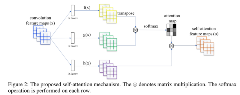
The resulting tensor is linearly-combined with h and, finally, scaled by gamma. Note that gamma starts as 0.
At the beginning of training, gamma cancels out the attention layers. As a consequence, the network only relies on local representations from the regular convolutional layers. However, as gamma receives gradient descent updates, the network gradually allows the passage of signals from non-local fields.
Also, note that the feature vectors f and g have different dimensions to h. As a matter of fact, f and g use eight times fewer convolutional filters than h.
This is the complete code for the self attention module:
Spectral normalization
Previously, Miyato et al proposed a normalization technique called spectral normalization (SN). In a few words, SN constrains the Lipschitz constant of the convolutional filters. The authors used SN as a way to stabilize the training of the D network. In practice, it worked very well.
Yet, there is one fundamental problem when training a normalized D. Prior work has shown that regularized D make the GAN training slower. For this reason, some workarounds consist of uneven rates of update steps between G and D. In other words, we can update D a few times before updating G. For instance, a regularized D might require five or more update steps for one G update.
To solve the problem of slow learning and imbalanced update steps, there is a simple yet effective approach. It is important to note that, in the GAN framework, G and D train together. In this context, Heusel et al introduced the two-timescale update rule (TTUR) in the GAN training. It consists of providing different learning rates for optimizing G and D.
Here, D trains with a learning rate four times greater than G — 0.004 and 0.001, respectively. A larger learning rate means that D will absorb a larger part of the gradient signal. Hence, a higher learning rate eases the problem of slow learning of the regularized D. Also, this approach makes it possible to use the same rate of updates for G and D. In fact, we use a 1:1 update interval between G and D.
Moreover, this paper has shown that well-conditioned generators are causally related to GAN performance. Given that, Self-Attention for GANs proposed using SN for stabilizing training of the generator network as well. For G, spectral normalisation prevents the parameters getting very big, and avoids unwanted gradients.
Implementation
It is important to note that the SN algorithm introduced by Miyato et al is an iterative approximation. It defines that, for each layer W, the spectral norm used to regularize each Convolutional layer W it the largest singular value of W.
However, applying singular value decomposition at each step might be computationally expansive. Instead, Miyato et al uses the power iteration method to estimate the SN of each layer.
To implement SN using Tensorflow eager execution with the Keras layers, we had to download and tweak the convolutions.py file. The complete code can be accessed here. Below we show the juicy parts of the algorithm.
To begin, we randomly initialize a vector u as following:
self.u = K.random_normal_variable([1, units], 0, 1, dtype=self.dtype)As shown in Algorithm 1 below, the power iteration method computes l2-distances between the linear combination of the vector u and the convolutional kernels Wi. Also, the SN is calculated on the unnormalized kernel weights.
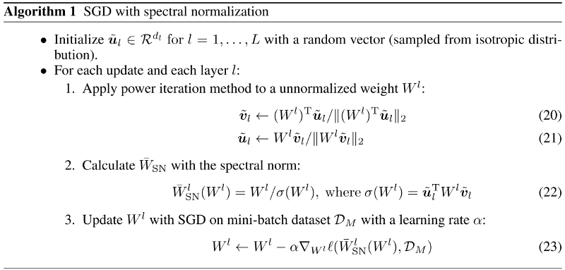
Note that, during training, the values of ũ, calculated in the power iteration, are used as the initial values of u in the next iteration. This strategy allows the algorithm to get very good estimates using only one round of the power iteration. Also, to normalize the kernel weights, we divide them by the current SN estimation.
Training details
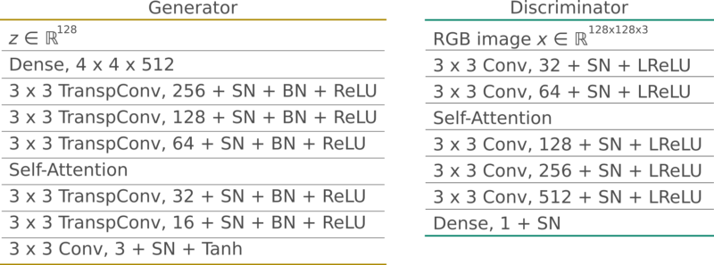
We trained a custom version of the SAGAN model using SN and self-attention. We used the Tensorflow’s tf.keras module and the Eager execution API.
G takes a random vector z and generates 128x128 RGB images. All layers, including dense layers, use SN. Additionally, G uses batch normalization and ReLU activations. Also, it uses self-attention in between middle-to-high feature maps. Like in the original implementation, we placed the attention layer to act on feature maps with dimensions 32x32.
D also uses spectral normalization (all layers). It takes RGB image samples of size 128x128 and outputs an unscaled probability. It uses leaky ReLUs with an alpha parameter of 0.02. Like G, it has a self-attention layer operating with feature maps of dimensions 32x32.
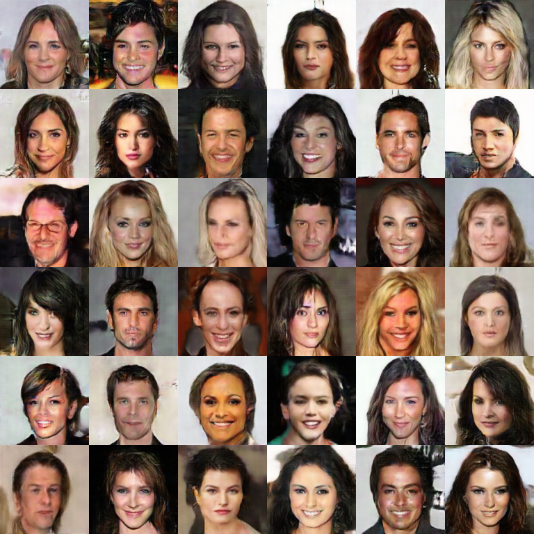
The goal is to minimize the hinge version of the adversarial loss. To do that, we trained G and D in an alternating fashion, using the Adam Optimizer, for 200 training steps.

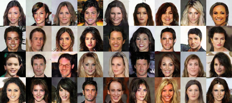
For this task, we used the Large-scale CelebFaces Attributes (CelebA) Dataset.
These are the results.
Thanks for reading!

Originally published at sthalles.github.io.