Everything you need to know to master Convolutional Neural Networks

by Tirmidzi Faizal Aflahi

Look at the photo below:

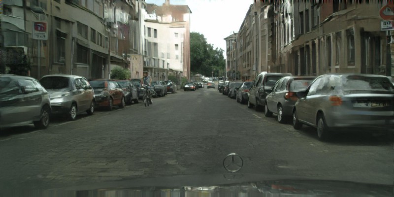
That is not a real photo. You can open the image in a new tab and zoom into the image. Do you see the mosaics?

The picture is actually generated by a program called Artificial Intelligence. Doesn’t it feel realistic? It’s great, isn’t it?

It has been only 7 years since the technology was brought to the public by Alex Krizhevsky and friends via the ImageNet competition. This competition is an annual Computer Vision competition to categorize pictures into 1000 different classes. From Alaskan Malamutes to toilet paper. Alex and friends built something called AlexNet, and it won the competition with a large margin between it and second place.

This technology is called a Convolutional Neural Network. It’s a sub-branch of Deep Neural Networks which performs exceptionally well in processing images.

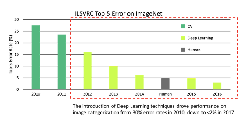
The image above is the error rate produced by the software that won the competition several years back. In 2016, it is actually better than human performance which was around 5%.

The introduction of Deep Learning into this field is actually game breaking more than game-changing.

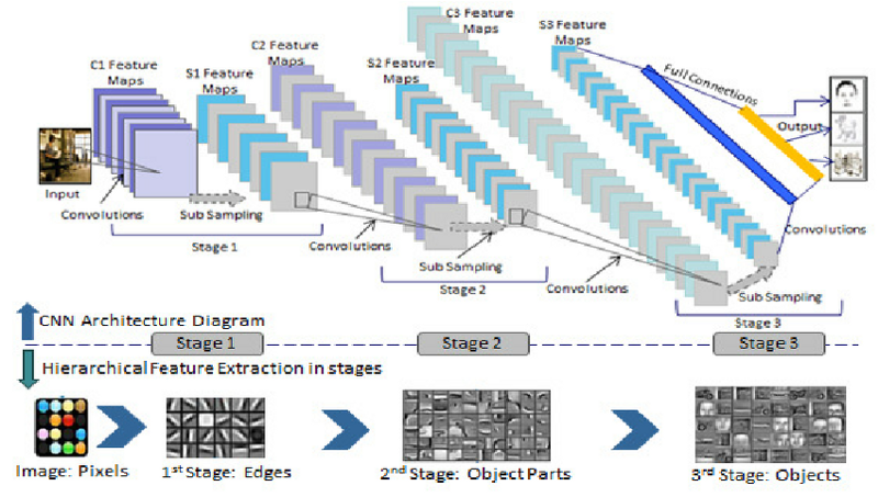
Convolutional Neural Network Architecture

So, how does this technology work?

Convolutional Neural Networks perform better than other Deep Neural Network architectures because of their unique process. Instead of looking at the image one pixel at a time, CNNs group several pixels together (an example 3×3 pixel like in the image above) so they can understand a temporal pattern.

In another way, CNNs can “see” group of pixels forming a line or curve. Because of the deep nature of Deep Neural Networks, in the next level they will see not the group of pixels, but groups of lines and curves forming some shapes. And so on until they form a complete picture.

There are many things you need to learn if you want to understand CNNs, from the very basic things, like a kernel, pooling layers, and so on. But nowadays, you can just dive and use many open source projects for this technology.

This is actually true because of the technology called Transfer Learning.

Transfer Learning

Transfer Learning is a technique which reuses the finished Deep Learning model in another more specific task.

As an example, say you are working in a Train Management company, and want to assess whether your trains are on time or not. And you don’t want to add another workforce just for this task.

You can just reuse an ImageNet Convolutional Neural Network model, maybe ResNet (the 2015 winner) and re-train the network with the images of your train fleets. And you will do just fine.

There are two main competitive edges when you use Transfer Learning.

1. Needs fewer images to perform well than training from scratch. ImageNet competition has around 1 million images to train with. Using transfer learning, you can use only 1000 or even 100 images and perform well because it is already trained with those 1 million images.
2. Needs less time to achieve good performance. To be as good as ImageNet, you will need to train the network for days, and that doesn’t count the time needed to alter the network if it doesn’t work well. Using transfer learning, you will only need several hours or even minutes to finish training for some tasks. A lot of time saved.

Image Classification to Image Generation

Enabled with transfer learning, many initiatives appeared. If you can process some images and tell us about what the images are all about, how about constructing the image itself?

Challenge accepted!

Generative Adversarial Network comes to the scene.

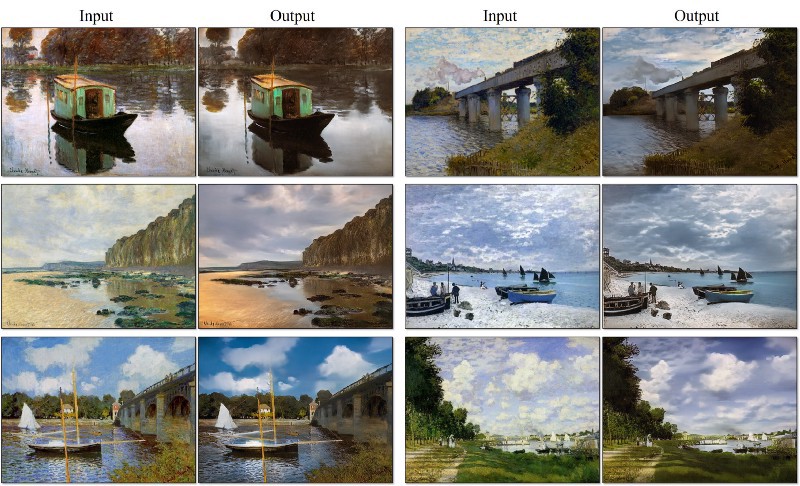
This technology can generate pictures using some inputs.

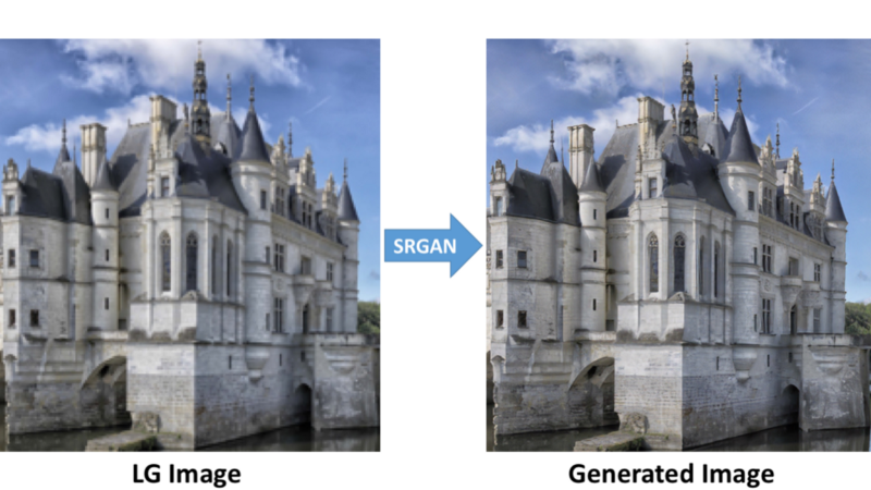
It can generate a realistic photo given a painting in a type called CycleGAN which I give you in the photo above. In another use case, it also can generate a picture of a bag given some sketches. It can even generate a higher resolution photo given a low-res photo.

Amazing, aren’t they?

Of course. And you can start learning to build them now. But how?

Convolutional Neural Network Tutorial

So, let’s begin. You will learn that getting started on this topic is easy, so freaking easy. But mastering it is on another level.

Let’s put aside mastering it for now.

After browsing for several days, I found this project which is really suitable for you to start with.

Aerial Cactus Identification

This is a tutorial project from Kaggle. Your task is to identify is there any columnar cactus in an aerial image

Pretty simple, eh?

You will be given 17,500 images to work with and need to label 4,000 images that have not been labeled. Your score is 1 or 100% if all the 4,000 images are correctly labeled by your program.

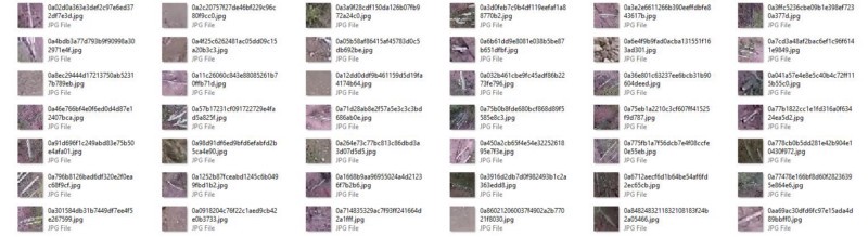
The images are pretty much like what you see above. A photo of a region that may or may not contains a group of columnar cacti. The photos are 32×32 pixels. And it shows cacti in different directions since they are aerial photos.

So what do you need?

Convolutional Neural Network with Python

Yes, Python, the popular language for Deep Learning. With many choices available, you can practically do trial and error for each choice. The choices are:

1. Tensorflow, the most popular Deep Learning library. Built by engineers at Google and has the biggest contributor base and most fans. Because the community is so big, you can easily find the solution to your problem. It has Keras as the high-level abstraction wrapper, that is so favorable for a newbie.
2. Pytorch. My favorite Deep Learning library. Built purely on Python and following the pros and cons of Python. Python developers will be extremely familiar with this library. It has another library called FastAI which gives the abstraction Keras has for Tensorflow.
3. MXNet. The Deep Learning library by Apache.
4. Theano. Predecessor of Tensorflow
5. CNTK. Microsoft also has his own Deep Learning library.

For this tutorial, let’s use my favorite one, Pytorch, complemented by its abstraction, FastAI.

Before starting, you need to install Python. Go to the Python website and download what you need. You need to make sure that you install version 3.6+, or it may not be supported by the libraries you will use.

Now, open your command line or terminal and install these things

pip install numpy pip install pandas pip install jupyter

Numpy will be used to store the inputted images. And pandas to work with CSV files. Jupyter notebook is what you need to interactively code with Python.

Then, go to the Pytorch website and download what you need. You might need the CUDA version to fasten your training speed. But make sure that you have version 1.0+ for Pytorch.

After that, install torchvision and FastAI:

pip install torchvision pip install fastai

Run Jupyter with the command jupyter notebook and it will open a browser window.

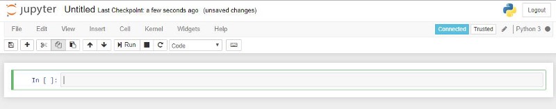
Now, you are ready to go.

Prepare the Data

Import the necessary code:

import numpy as npimport pandas as pd from pathlib import Path from fastai import * from fastai.vision import * import torch %matplotlib inline

Numpy and Pandas are always needed for everything you want to do. FastAI and Torch are your Deep Learning Library. Matplotlib Inline will be used to show charts.

Now, download data files from the competition website.

Extract the zip data file and put them inside the jupyter notebook folder.

Let’s say you named your notebook Cacti. Your folder structure would be like this:

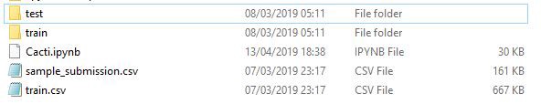
Train folder contains all the images for your training step.

Test folder contains all the images for submission.

Train CSV file contains the training data; mapping the image name with the column has_cactus which gives a value of 1 if it has cactus or 0 otherwise.

Sample Submission CSV file contains all the formatting for submission that you need to do. The file names stated there are equal to all files inside Test folder.

train_df = pd.read_csv("train.csv")

Load the Train CSV file to a data frame.

data_folder = Path(".") train_images = ImageList.from_df(train_df, path=data_folder, folder='train')

Create a load generator using the ImageList from_df method to map train_df data frame with images inside the train folder.

Data Augmentation

This is a technique to create more data from your existing data. An image of a cat flipped vertically is still a cat. By doing this you can basically multiply your data set twice, four times, or even 16 times.

You will need this technique a lot if you happen to have very little data to work with.

transformations = get_transforms(do_flip=True, flip_vert=True, max_rotate=10.0, max_zoom=1.1, max_lighting=0.2, max_warp=0.2, p_affine=0.75, p_lighting=0.75)

FastAI gives you a nice transformation method to do all of this, called get_transform. You can do a flip vertically, horizontally, rotate, zoom, add lighting/brightness, and warp the image.

You can play with the parameter I stated above to find out how it will look. Or you can open the documentation and read about it in detail.

Of course, apply the transformation to your image list:

train_img = train_img.transform(transformations, size=128)

The parameter size will be used to scale up or down the input to match with the neural network you will use. The network I will use is called DenseNet, which won Best Paper Award at ImageNet 2017, and it needs images with 128×128 pixels in size.

Training Preparation

After loading your data, you need to prepare yourself and your data for the most important phase in Deep Learning called Training. Basically, this is the Learning in Deep Learning. It learns from your data, and updates itself accordingly so that it will have good performance on your data.

test_df = pd.read_csv("sample_submission.csv") test_img = ImageList.from_df(test_df, path=data_folder, folder='test')

train_img = train_img           .split_by_rand_pct(0.01)           .label_from_df()           .add_test(test_img)           .databunch(path='.', bs=64, device=torch.device('cuda:0'))                       .normalize(imagenet_stats)

For the training step, you need to split some of your training data into a small portion called validation data. You can’t touch these data because they will be your validation tool. When your Convolutional Neural Network performs well on validation data, it will likely perform well on the test data that will be submitted.

FastAI has the convenient method called split_by_rand_pct to split a portion of your data into validation data.

It also has the method databunch to perform batch processing. I used 64 as the batch because that is what my GPU limits. If you don’t have GPU, emit the device parameter.

Then, the normalize method is called to normalize your images because you will use a pre-trained network. imagenet_stats will normalize the images according to how the pre-trained network was trained for the ImageNet competition.

Adding the test data to the training image list makes it easy to predict later on without more pre-processing. Remember, these images will not be trained on and will not go to your validation. You just want to pre-process the data in the same way with the training images.

learn = cnn_learner(train_img, models.densenet161, metrics=[error_rate, accuracy])

You are done preparing your training data. Now, create a training method with cnn_learner. As I said before, I will use DenseNet as the pre-trained network. You can use another network offered in TorchVision.

The One-Cycle Technique

You can start your training right now. But, there is always confusion when training any Deep Neural Network, Convolutional Neural Networks included. That is choosing the right learning rate. The algorithm is called Gradient Descent, and it will try to decrease the error defined with a parameter called learning rate.

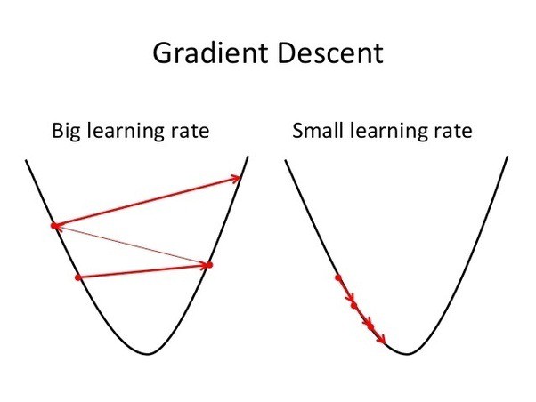
A bigger learning rate makes the training steps faster, but it is prone to overstepping the boundaries. This makes it possible for the error to go out of control like the picture above. While a smaller learning rate makes the training steps slower, but it will not go out of control.

So, choosing the right learning rate is really important. Make it big enough without going out of control.

It is easier said than done.

So, there came a person called Leslie Smith who create a technique called the 1-cycle policy.

Intuition wise, you might want to find / brute force several learning rates and find one with nearly minimal error but have some space to improve. Let’s try it out in our code.

learn.lr_find() learn.recorder.plot()

It will print something like this:

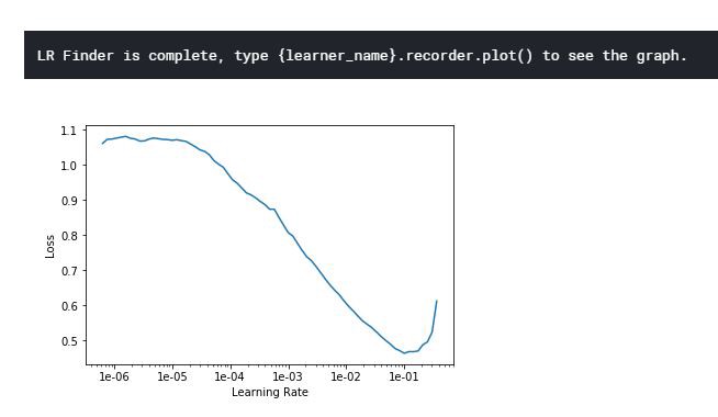
The minimum should be 10 ⁻¹. So, I think we can use something smaller than that but not too small. Maybe 3 * 10 ⁻ ² is a good choice. Let’s try it!

lr = 3e-02 learn.fit_one_cycle(5, slice(lr))

Train for several steps (I choose 5, not too big and not too small), and let’s see the result.

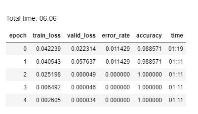
Wait, what!?

Our simple solution gives us 100% accuracy for our validation split! It is actually effective. And it only needs six minutes to train. What a stroke of luck! In real life, you will do several iterations just to find out which algorithms do better than the others.

I am eager to submit! Haha. Let’s predict the test folder and submit the result.

preds,_ = learn.get_preds(ds_type=DatasetType.Test) test_df.has_cactus = preds.numpy()[:, 0]

Because you have already put the test images in the training image list, you will not need to pre-process and load your test images.

test_df.to_csv('submission.csv', index=False)

This line will create a CSV file containing the images name and has a cactus column for all 4,000 test images.

When I tried to submit, I actually just realized that you need to submit the CSV via a Kaggle kernel. I missed that.

But, luckily, the kernel is actually the same as your jupyter notebook. You can just copy paste all the things you have built in your notebook and submit there.

And BAM!

Good Lord! I get 0.9999 for the public score. That’s really good. But, of course, I want to get a perfect score if my first attempt is like that.

So, I did several tweaks in the network and once more, BAM!

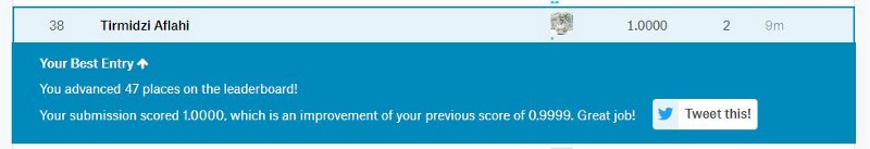
I did it! So can you. It’s actually not that hard.

(BTW, this rank was taken on April 13th, so I might drop my rank right by now…)

What I Learned

This problem is easy. So, you will not face any weird challenge while solving it. This makes it one of the most suitable projects to start with.

Alas, because many people get a perfect score on this, I think the admin needs to create another test set for submission. A harder one maybe.

Whatever the reason, there is no barrier for you to try this. You can try this right now and get good results.

Final Thoughts

Convolutional Neural Networks are so helpful for various tasks. From Image Recognition to generating images. Analyzing images nowadays is not as hard as before. Of course, you can also do it if you try.

Just get started, pick a good Convolutional Neural Network project, and get good data.

Good luck!

This article is originally published on my blog at thedatamage.