
by Sterling Osborne, PhD Researcher
How to apply Reinforcement Learning to real life planning problems

Recently, I have published some examples where I have created Reinforcement Learning models for some real life problems. For example, using Reinforcement Learning for Meal Planning based on a Set Budget and Personal Preferences.
Reinforcement Learning can be used in this way for a variety of planning problems including travel plans, budget planning and business strategy. The two advantages of using RL is that it takes into account the probability of outcomes and allows us to control parts of the environment. Therefore, I decided to write a simple example so others may consider how they could start using it to solve some of their day-to-day or work problems.
What is Reinforcement Learning?
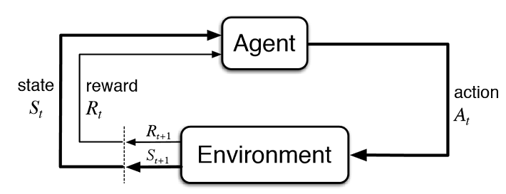
Reinforcement Learning (RL) is the process of testing which actions are best for each state of an environment by essentially trial and error. The model introduces a random policy to start, and each time an action is taken an initial amount (known as a reward) is fed to the model. This continues until an end goal is reached, e.g. you win or lose the game, where that run (or episode) ends and the game resets.
As the model goes through more and more episodes, it begins to learn which actions are more likely to lead us to a positive outcome. Therefore it finds the best actions in any given state, known as the optimal policy.
Many of the RL applications online train models on a game or virtual environment where the model is able to interact with the environment repeatedly. For example, you let the model play a simulation of tic-tac-toe over and over so that it observes success and failure of trying different moves.
In real life, it is likely we do not have access to train our model in this way. For example, a recommendation system in online shopping needs a person’s feedback to tell us whether it has succeeded or not, and this is limited in its availability based on how many users interact with the shopping site.
Instead, we may have sample data that shows shopping trends over a time period that we can use to create estimated probabilities. Using these, we can create what is known as a Partially Observed Markov Decision Process (POMDP) as a way to generalise the underlying probability distribution.
Partially Observed Markov Decision Processes (POMDPs)
Markov Decision Processes (MDPs) provide a framework for modeling decision making in situations where outcomes are partly random and partly under the control of a decision maker. The key feature of MDPs is that they follow the Markov Property; all future states are independent of the past given the present. In other words, the probability of moving into the next state is only dependent on the current state.
POMDPs work similarly except it is a generalisation of the MDPs. In short, this means the model cannot simply interact with the environment but is instead given a set probability distribution based on what we have observed. More info can be found here. We could use value iteration methods on our POMDP, but instead I’ve decided to use Monte Carlo Learning in this example.
Example Environment
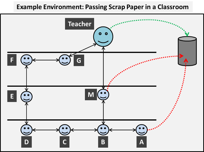
Imagine you are back at school (or perhaps still are) and are in a classroom, the teacher has a strict policy on paper waste and requires that any pieces of scrap paper must be passed to him at the front of the classroom and he will place the waste into the bin (trash can).
However, some students in the class care little for the teacher’s rules and would rather save themselves the trouble of passing the paper round the classroom. Instead, these troublesome individuals may choose to throw the scrap paper into the bin from a distance. Now this angers the teacher and those that do this are punished.
This introduces a very basic action-reward concept, and we have an example classroom environment as shown in the following diagram.
Our aim is to find the best instructions for each person so that the paper reaches the teacher and is placed into the bin and avoids being thrown in the bin.
States and Actions
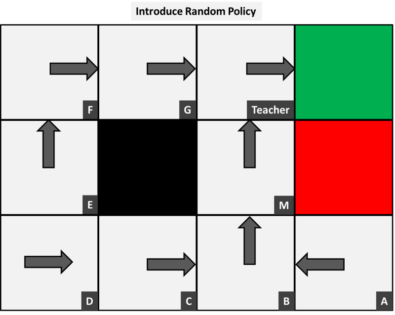
In our environment, each person can be considered a state and they have a variety of actions they can take with the scrap paper. They may choose to pass it to an adjacent class mate, hold onto it or some may choose to throw it into the bin. We can therefore map our environment to a more standard grid layout as shown below.

This is purposefully designed so that each person, or state, has four actions: up, down, left or right and each will have a varied ‘real life’ outcome based on who took the action. An action that puts the person into a wall (including the black block in the middle) indicates that the person holds onto the paper. In some cases, this action is duplicated, but is not an issue in our example.
For example, person A’s actions result in:
- Up = Throw into bin
- Down = Hold onto paper
- Left = Pass to person B
- Right = Hold onto paper
Probabilistic Environment
For now, the decision maker that partly controls the environment is us. We will tell each person which action they should take. This is known as the policy.
The first challenge I face in my learning is understanding that the environment is likely probabilistic and what this means. A probabilistic environment is when we instruct a state to take an action under our policy, there is a probability associated as to whether this is successfully followed. In other words, if we tell person A to pass the paper to person B, they can decide not to follow the instructed action in our policy and instead throw the scrap paper into the bin.
Another example is if we are recommending online shopping products there is no guarantee that the person will view each one.
Observed Transitional Probabilities
To find the observed transitional probabilities, we need to collect some sample data about how the environment acts. Before we collect information, we first introduce an initial policy. To start the process, I have randomly chosen one that looks as though it would lead to a positive outcome.
Now we observe the actions each person takes given this policy. In other words, say we sat at the back of the classroom and simply observed the class and observed the following results for person A:
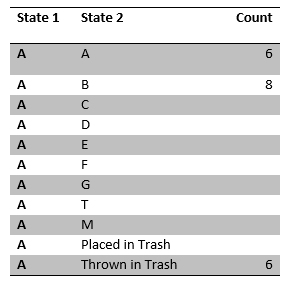
We see that a paper passed through this person 20 times; 6 times they kept hold of it, 8 times they passed it to person B and another 6 times they threw it in the trash. This means that under our initial policy, the probability of keeping hold or throwing it in the trash for this person is 6/20 = 0.3 and likewise 8/20 = 0.4 to pass to person B. We can observe the rest of the class to collect the following sample data:
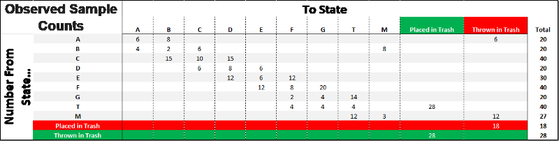
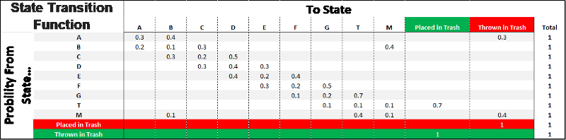
Likewise, we then calculate the probabilities to be the following matrix and we could use this to simulate experience. The accuracy of this model will depend greatly on whether the probabilities are true representations of the whole environment. In other words, we need to make sure we have a sample that is large and rich enough in data.
Multi-Armed Bandits, Episodes, Rewards, Return and Discount Rate
So we have our transition probabilities estimated from the sample data under a POMDP. The next step, before we introduce any models, is to introduce rewards. So far, we have only discussed the outcome of the final step; either the paper gets placed in the bin by the teacher and nets a positive reward or gets thrown by A or M and nets a negative rewards. This final reward that ends the episode is known as the Terminal Reward.
But, there is also third outcome that is less than ideal either; the paper continually gets passed around and never (or takes far longer than we would like) reaches the bin. Therefore, in summary we have three final outcomes
- Paper gets placed in bin by teacher and nets a positive terminal reward
- Paper gets thrown in bin by a student and nets a negative terminal reward
- Paper gets continually passed around room or gets stuck on students for a longer period of time than we would like
To avoid the paper being thrown in the bin we provide this with a large, negative reward, say -1, and because the teacher is pleased with it being placed in the bin this nets a large positive reward, +1. To avoid the outcome where it continually gets passed around the room, we set the reward for all other actions to be a small, negative value, say -0.04.
If we set this as a positive or null number then the model may let the paper go round and round as it would be better to gain small positives than risk getting close to the negative outcome. This number is also very small as it will only collect a single terminal reward but it could take many steps to end the episode and we need to ensure that, if the paper is place in the bin, the positive outcome is not cancelled out.
Please note: the rewards are always relative to one another and I have chosen arbitrary figures, but these can be changed if the results are not as desired.
Although we have inadvertently discussed episodes in the example, we have yet to formally define it. An episode is simply the actions each paper takes through the classroom reaching the bin, which is the terminal state and ends the episode. In other examples, such as playing tic-tac-toe, this would be the end of a game where you win or lose.
The paper could in theory start at any state and this introduces why we need enough episodes to ensure that every state and action is tested enough so that our outcome is not being driven by invalid results. However, on the flip side, the more episodes we introduce the longer the computation time will be and, depending on the scale of the environment, we may not have an unlimited amount of resources to do this.
This is known as the Multi-Armed Bandit problem; with finite time (or other resources), we need to ensure that we test each state-action pair enough that the actions selected in our policy are, in fact, the optimal ones. In other words, we need to validate that actions that have lead us to good outcomes in the past are not by sheer luck but are in fact in the correct choice, and likewise for the actions that appear poor. In our example this may seem simple with how few states we have, but imagine if we increased the scale and how this becomes more and more of an issue.
The overall goal of our RL model is to select the actions that maximises the expected cumulative rewards, known as the return. In other words, the Return is simply the total reward obtained for the episode. A simple way to calculate this would be to add up all the rewards, including the terminal reward, in each episode.
A more rigorous approach is to consider the first steps to be more important than later ones in the episode by applying a discount factor, gamma, in the following formula:
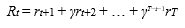
In other words, we sum all the rewards but weigh down later steps by a factor of gamma to the power of how many steps it took to reach them.
If we think about our example, using a discounted return becomes even clearer to imagine as the teacher will reward (or punish accordingly) anyone who was involved in the episode but would scale this based on how far they are from the final outcome.
For example, if the paper passed from A to B to M who threw it in the bin, M should be punished most, then B for passing it to him and lastly person A who is still involved in the final outcome but less so than M or B. This also emphasises that the longer it takes (based on the number of steps) to start in a state and reach the bin the less is will either be rewarded or punished but will accumulate negative rewards for taking more steps.
Applying a Model to our Example
As our example environment is small, we can apply each and show some of the calculations performed manually and illustrate the impact of changing parameters.
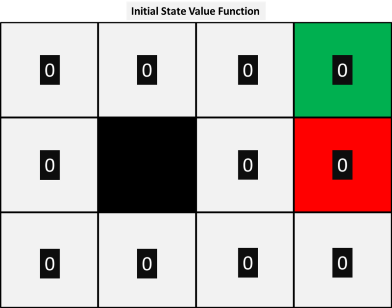
For any algorithm, we first need to initialise the state value function, V(s), and have decided to set each of these to 0 as shown below.
Next, we let the model simulate experience on the environment based on our observed probability distribution. The model starts a piece of paper in random states and the outcomes of each action under our policy are based on our observed probabilities. So for example, say we have the first three simulated episodes to be the following:
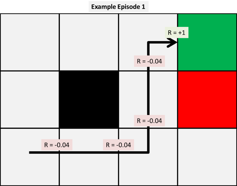
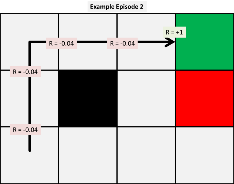

With these episodes we can calculate our first few updates to our state value function using each of the three models given. For now, we pick arbitrary alpha and gamma values to be 0.5 to make our hand calculations simpler. We will show later the impact this variable has on results.
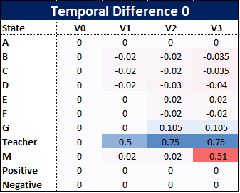
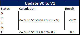
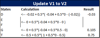
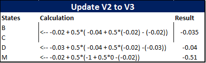
First, we apply temporal difference 0, the simplest of our models and the first three value updates are as follows:
So how have these been calculated? Well because our example is small we can show the calculations by hand.
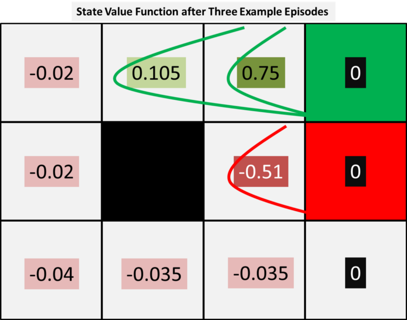
So what can we observe at this early stage? Firstly, using TD(0) appears unfair to some states, for example person D, who, at this stage, has gained nothing from the paper reaching the bin two out of three times. Their update has only been affected by the value of the next stage, but this emphasises how the positive and negative rewards propagate outwards from the corner towards the states.
As we take more episodes the positive and negative terminal rewards will spread out further and further across all states. This is shown roughly in the diagram below where we can see that the two episodes the resulted in a positive result impact the value of states Teacher and G whereas the single negative episode has punished person M.
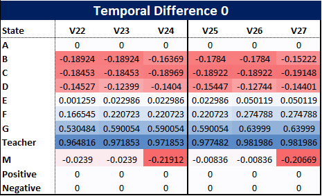
To show this, we can try more episodes. If we repeat the same three paths already given we produce the following state value function:
(Please note, we have repeated these three episodes for simplicity in this example but the actual model would have episodes where the outcomes are based on the observed transition probability function.)
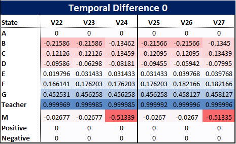
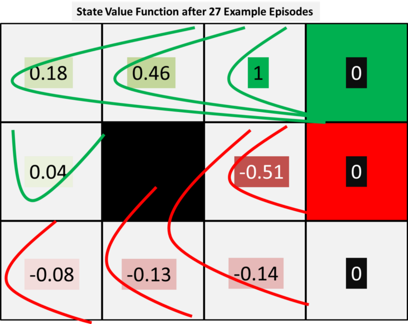
The diagram above shows the terminal rewards propagating outwards from the top right corner to the states. From this, we may decide to update our policy as it is clear that the negative terminal reward passes through person M and therefore B and C are impacted negatively. Therefore, based on V27, for each state we may decide to update our policy by selecting the next best state value for each state as shown in the figure below
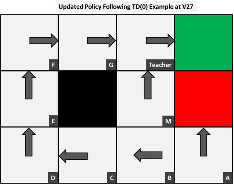
There are two causes for concerns in this example: the first is that person A’s best action is to throw it into the bin and net a negative reward. This is because none of the episodes have visited this person and emphasises the multi armed bandit problem. In this small example there are very few states so would require many episodes to visit them all, but we need to ensure this is done.
The reason this action is better for this person is because neither of the terminal states have a value but rather the positive and negative outcomes are in the terminal rewards. We could then, if our situation required it, initialise V0 with figures for the terminal states based on the outcomes.
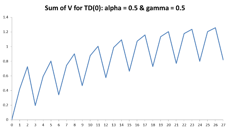
Secondly, the state value of person M is flipping back and forth between -0.03 and -0.51 (approx.) after the episodes and we need to address why this is happening. This is caused by our learning rate, alpha. For now, we have only introduced our parameters (the learning rate alpha and discount rate gamma) but have not explained in detail how they will impact results.
A large learning rate may cause the results to oscillate, but conversely it should not be so small that it takes forever to converge. This is shown further in the figure below that demonstrates the total V(s) for every episode and we can clearly see how, although there is a general increasing trend, it is diverging back and forth between episodes. Another good explanation for learning rate is as follows:
“In the game of golf when the ball is far away from the hole, the player hits it very hard to get as close as possible to the hole. Later when he reaches the flagged area, he chooses a different stick to get accurate short shot.
So it’s not that he won’t be able to put the ball in the hole without choosing the short shot stick, he may send the ball ahead of the target two or three times. But it would be best if he plays optimally and uses the right amount of power to reach the hole.”
Learning rate of a Q learning agent
The question how the learning rate influences the convergence rate and convergence itself. If the learning rate is…stackoverflow.com
There are some complex methods for establishing the optimal learning rate for a problem but, as with any machine learning algorithm, if the environment is simple enough you iterate over different values until convergence is reached. This is also known as stochastic gradient decent. In a recent RL project, I demonstrated the impact of reducing alpha using an animated visual and this is shown below. This demonstrates the oscillation when alpha is large and how this becomes smoothed as alpha is reduced.
Likewise, we must also have our discount rate to be a number between 0 and 1, oftentimes this is taken to be close to 0.9. The discount factor tells us how important rewards in the future are; a large number indicates that they will be considered important whereas moving this towards 0 will make the model consider future steps less and less.
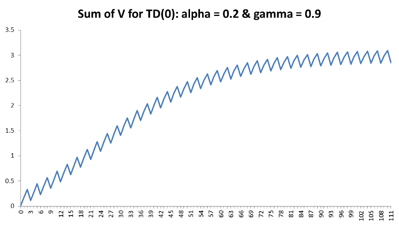
With both of these in mind, we can change both alpha from 0.5 to 0.2 and gamma from 0.5 to 0.9 and we achieve the following results:
Because our learning rate is now much smaller the model takes longer to learn and the values are generally smaller. Most noticeably is for the teacher which is clearly the best state. However, this trade-off for increased computation time means our value for M is no longer oscillating to the degree they were before. We can now see this in the diagram below for the sum of V(s) following our updated parameters. Although it is not perfectly smooth, the total V(s) slowly increases at a much smoother rate than before and appears to converge as we would like but requires approximately 75 episodes to do so.
Changing the Goal Outcome
Another crucial advantage of RL that we haven’t mentioned in too much detail is that we have some control over the environment. Currently, the rewards are based on what we decided would be best to get the model to reach the positive outcome in as few steps as possible.
However, say the teacher changed and the new one didn’t mind the students throwing the paper in the bin so long as it reached it. Then we can change our negative reward around this and the optimal policy will change.
This is particularly useful for business solutions. For example, say you are planning a strategy and know that certain transitions are less desired than others, then this can be taken into account and changed at will.
Conclusion
We have now created a simple Reinforcement Learning model from observed data. There are many things that could be improved or taken further, including using a more complex model, but this should be a good introduction for those that wish to try and apply to their own real-life problems.
I hope you enjoyed reading this article, if you have any questions please feel free to comment below.
Thanks
Sterling