by Wolfgang Beyer
How to Build a Simple Image Recognition System with TensorFlow (Part 2)
This is the second part of my introduction to building an image recognition system with TensorFlow. In the first part we built a softmax classifier to label images from the CIFAR-10 dataset. We achieved an accuracy of around 25–30%. Since there are 10 different and equally likely categories, labeling the images randomly we’d expect an accuracy of 10%. So we’re already a lot better than random, but there’s still plenty of room for improvement.
In this post, I’ll describe how to build a neural network that performs the same task. Let’s see by how much we can increase our prediction accuracy!
Neural Networks
Neural networks are very loosely based on how biological brains work. They consist of a number of artificial neurons which each process multiple incoming signals and return a single output signal. The output signal can then be used as an input signal for other neurons.
Let’s take a look at an individual neuron:
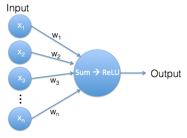
What happens in a single neuron is very similar to what happens in the the softmax classifier. Again we have a vector of input values and a vector of weights. The weights are the neuron’s internal parameters. Both input vector and weights vector contain the same number of values, so we can use them to calculate a weighted sum.

So far, we’re doing exactly the same calculation as in the softmax classifier, but now comes a little twist: as long as the result of the weighted sum is a positive value, the neuron’s output is this value. But if the weighted sum is a negative value, we ignore that negative value and the neuron generates an output of 0 instead. This operation is called a Rectified Linear Unit (ReLU).
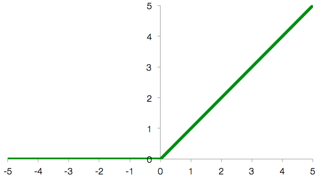
The reason for using a ReLU is that this creates a nonlinearity. The neuron’s output is now not strictly a linear combination (= weighted sum) of its inputs anymore. We’ll see why this is useful when we stop looking at individual neurons and instead look at the whole network.
The neurons in artificial neural networks are usually not connected randomly to each other. Most of the time they are arranged in layers:
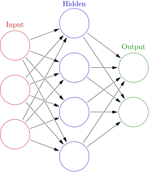
(Image is part of the Wikimedia Commons and was taken from here)
The input image’s pixel values are the inputs for the network’s first layer of neurons. The output of the neurons in layer 1 is the input for neurons of layer 2 and so forth. This is the reason why having a nonlinearity is so important. Without the ReLU at each layer, we would only have a sequence of weighted sums. And stacked weighted sums can be merged into a single weighted sum, so the multiple layers would give us no improvement over a single layer network. Introducing the ReLU nonlinearity solves this problem as each additional layer really adds something to the network.
The network’s final layer’s output are the values we are interested in, the scores for the image categories. In this network architecture each neuron is connected to all neurons of the previous layer, therefore this kind of network is called a fully connected network. As we shall see in Part 3 of this Tutorial, that is not necessarily always the case.
And that’s already the end of my very brief part on the theory of neural networks. Let’s get started building one!
The Code
The full code for this example is available on Github. It requires TensorFlow and the CIFAR-10 dataset (see Part 1) on how to install the prerequisites).
If you’ve made your way through my previous blog post, you’ll see that the code for the neural network classifier is pretty similar to the code for the softmax classifier. But in addition to switching out the part of the code that defines the model, I’ve added a couple of small features to show some of the things TensorFlow can do:
- Regularization: this is a very common technique to prevent overfitting of a model. It works by applying a counter-force during the optimization process which aims to keep the model simple.
- Visualization of the model with TensorBoard: TensorBoard is included with TensorFlow and allows you to generate charts and graphs from your models and from data generated by your models. This helps with analyzing your models and is especially useful for debugging.
- Checkpoints: this feature allows you to save the current state of your model for later use. Training a model can take quite a while, so it’s essential to not have to start from scratch each time you want to use it.
The code is split into two files this time: there’s two_layer_fc.py, which defines the model, and run_fc_model.py, which runs the model (in case you’re wondering: ‘fc’ stands for fully connected).
2-Layer Fully Connected Neural Network
Let’s look at the model itself first and deal with running and training it later. two_layer_fc.py contains the following functions:
inference()gets us from input data to class scores.loss()calculates the loss value from class scores.training()performs a single training step.evaluation()calculates the accuracy of the network.
Generating Class Scores: inference()
inference() describes the forward pass through the network. How are the class scores calculated, starting from input images?
The images parameter is the TensorFlow placeholder containing the actual image data. The next three parameters describe the shape/size of the network. image_pixels is the number of pixels per input image, classes is the number of different output labels and hidden_units is the number of neurons in the first/hidden layer of our network.
Each neuron takes all values from the previous layer as input and generates a single output value. Each neuron in the hidden layer therefore has image_pixels inputs and the layer as a whole generates hidden_units outputs. These are then fed into the classes neurons of the output layer which generate classes output values, one score per class.
reg_constant is the regularization constant. TensorFlow allows us to add regularization to our network very easily by handling most of the calculations automatically. I’ll go into a bit more detail when we get to the loss function.
Since our neural network has 2 similar layers, we’ll define a separate scope for each. This allows us to reuse variable names in each scope. The biases variable is defined in the way we already know, by using tf.Variable().
The definition of the weights variable is a bit more involved. We use tf.get_variable(), which allows us to add regularization. weights is a matrix with dimensions of image_pixels by hidden_units (input vector size x output vector size). The initializer parameter describes the weight variable’s initial values.
Up to now, we’ve initialized our variables to 0, but this wouldn’t work here. Think about the neurons in a single layer. They all receive exactly the same input values. If they all had the same internal parameters as well, they would all make the same calculation and all output the same value. To avoid this, we need to randomize their initial weights. We use an initialization scheme which usually works well, the weights are initialized to normally distributed values. We drop values which are more than 2 standard deviations from the mean, and the standard deviation is set to the inverse of the square root of the number of input pixels. Luckily TensorFlow handles all these details for us, we just need to specify that we want to use a truncated_normal_initializer which does exactly what we want.
The final parameter for the weights variable is the regularizer. All we have to do at this point is to tell TensorFlow we want to use L2-regularization for the weights variable. I’ll cover regularization here.
To create the first layer’s output we multiply the images matrix and the weights matrix witch each other and add the bias variable. This is exactly the same as in the softmax classifier from the previous blog post. Then we apply tf.nn.relu(), the ReLU function to arrive at the hidden layer’s output.
Layer 2 is very similar to layer 1. The number of inputs is hidden_units, the number of outputs is classes. Therefore the dimensions of the weights matrix are [hidden_units, classes]. Since this is the final layer of our network, there’s no need for a ReLU anymore. We arrive at the class scores (logits) by multiplying input (hidden) and weights with each other and adding bias.
The summary operation tf.histogram_summary() allows us to record the value of the logits variable for later analysis with TensorBoard. I’ll cover this later.
To sum it up, the inference() function as whole takes in input images and returns class scores. That’s all a trained classifier needs to do, but in order to arrive at a trained classifier, we first need to measure how good those class scores are. That’s the job of the loss function.
Calculating the Loss: loss()
First we calculate the cross-entropy between logits(the model’s output) and labels(the correct labels from the training dataset). That has been our whole loss function for the softmax classifier, but this time we want to use regularization, so we have to add another term to our loss.
Let’s take a step back first and look at what we want to achieve by using regularization.
Overfitting and Regularization
When a statistical model captures the random noise in the data it was trained on instead of the true underlying relationship, this is called overfitting.
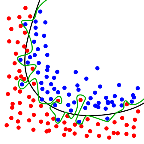
(Image is part of the Wikimedia Commons and was taken from here)
In the above image there are two different classes, represented by the blue and red circles. The green line is an overfitted classifier. It follows the training data perfectly, but it is also heavily dependent on it and is likely to handle unseen data worse than the black line, which represents a regularized model.
So our goal for regularization is to arrive at a simple model without any unnecessary complications. There are different ways to achieve this, and the option we are choosing is called L2-regularization. L2-regularization adds the sum of the squares of all the weights in the network to the loss function. This corresponds to a heavy penalty if the model is using big weights and a small penalty if the model is using small weights.
That’s why we used the regularizer parameter when defining the weights and assigned a l2_regularizer to it. This tells TensorFlow to keep track of the L2-regularization terms (and weigh them by the parameter reg_constant) for this variable. All regularization terms are added to a collection called tf.GraphKeys.REGULARIZATION_LOSSES, which the loss function accesses. We then add the sum of all regularization losses to the previously calculated cross-entropy to arrive at the total loss of our model.
Optimizing the Variables: training()
global_step is a scalar variable which keeps track of how many training iterations have already been performed. When repeatedly running the model in our training loop, we already know this value. It’s the iteration variable of the loop. The reason we’re adding this value directly to the TensorFlow graph is that we want to be able to take snapshots of the model. And these snapshots should include information about how many training steps have already been performed.
The definition of the gradient descent optimizer is simple. We provide the learning rate and tell the optimizer which variable it is supposed to minimize. In addition, the optimizer automatically increments the global_step parameter with every iteration.
Measuring Performance: evaluation()
The calculation of the model’s accuracy is the same as in the softmax case: we compare the model’s predictions with true labels and calculate the frequency of how often the prediction is correct. We’re also interested in how the accuracy evolves over time, so we’re adding a summary operation which keeps track of the value of accuracy. We’ll cover this in the section about TensorBoard.
To summarize what we have done so far, we have defined the behavior of a 2-layer artificial neural network using 4 functions: inference() constitutes the forward pass through the network and returns class scores. loss() compares predicted and true class scores and generates a loss value. training() performs a training step and optimizes the model’s internal parameters and evaluation() measures the performance of our model.
Running the Neural Network
Now that the neural network is defined, let’s look at how run_fc_model.py runs, trains and evaluates the model.
After the obligatory imports we’re defining the model parameters as external flags. TensorFlow has its own module for command line parameters, which is a thin wrapper around Python’s argparse. We’re using it here for convenience, but you can just as well use argparse directly instead.
In the first couple of lines, the various command line parameters are being defined. The parameters for each flag are the flag’s name, its default value and a short description. Executing the file with the -h flag displays these descriptions.
The second block of lines calls the function which actually parses the command line parameters. Then the values of all parameters are printed to the screen.
Here we define constants for the number of pixels per image (32 x 32 x 3) and the number of different image categories. Then we start measuring the runtime by creating a timer.
We want to log some info about the training process and use TensorBoard to display that info. TensorBoard requires the logs for each run to be in a separate directory, so we’re adding date and time info to the name of the log directory.
load_data() loads the CIFAR-10 data and returns a dictionary containing separate training and test datasets.
Generate the TensorFlow Graph
We’re defining TensorFlow placeholders. When performing the actual calculations, these will be filled with training/testing data.
The images_placeholder has dimensions of batch size x pixels per image. A batch size of ‘None’ allows us to run the graph with different batch sizes (the batch size for training the net can be set via a command line parameter, but for testing we’re passing the whole test set as a single batch).
The labels_placeholder is a vector of integer values containing the correct class label, one per image in the batch.
Here we’re referencing the functions we covered earlier in two_layer_fc.py.
inference()gets us from input data to class scores.loss()calculates a loss value from class scores.training()performs a single training step.evaluation()calculates the accuracy of the network.
Defines a summary operation for TensorBoard (covered here).
Generates a saver object to save the model’s state at checkpoints (covered here).
We start the TensorFlow session and immediately initialize all variables. Then we create a summary writer which we will use to periodically save log information to disk.
These lines are responsible for generating batches of input data. Let’s pretend we have 100 training images and a batch size of 10. In the softmax example we just picked 10 random images for each iteration. This means that after 10 iterations each image will have been picked once on average(!). But in fact some images will have been picked multiple times while some images haven’t been part of any batch so far. As long as you repeat this often enough, it’s not that terrible that randomness causes some images to be part of the training batches somewhat more often than others.
But this time we want to improve the sampling process. What we do is we first shuffle the 100 images of the training dataset. The first 10 images of the shuffled data are our first batch, the next 10 images are our second batch and so forth. After 10 batches we’re at the end of our dataset and the process starts again. We shuffle the data another time and run through it from front to back. This guarantees that no image is being picked more often than any other while still ensuring that the order in which the images are returned is random.
In order to achieve this, the gen_batch() function in data_helpers() returns a Python generator, which returns the next batch each time it is evaluated. The details of how generators work are beyond the scope of this post (a good explanation can be found here). We’re using the Python’s built-in zip() function to generate a list of tuples of the from [(image1, label1), (image2, label2), ...], which is then passed to our generator function.
next(batches) returns the next batch of data. Since it’s still in the form of [(imageA, labelA), (imageB, labelB), ...], we need to unzip it first to separate images from labels, before filling feed_dict, the dictionary containing the TensorFlow placeholders, with a single batch of training data.
Every 100 iterations the model’s current accuracy is evaluated and printed to the screen. In addition, the summary operation is being run and its results are added to the summary_writer which is responsible for writing the summaries to disk. From there they can be read and displayed by TensorBoard (see this section).
This line runs the train_step operation (defined previously to call two_layer_fc.training(), which contains the actual instructions for the optimization of the variables).
When training a model takes a longer period of time, there is an easy way to save a snapshot of your progress. This allows you to come back later and restore the model in exactly the same state. All you need to do is to create a tf.train.Saver object (we did that earlier) and then call its save() method every time you want to take a snapshot.
Restoring a model is just as easy, just call the saver’s restore() method. There is a working code example showing how to do this in the file restore_model.pyin the github repository.
After the training is finished, the final model is evaluated on the test set (remember, the test set contains data that the model has not seen so far, allowing us to judge how well the model is able to generalize to new data).
Results
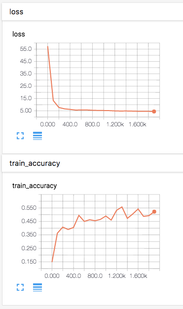
Let’s run the model with the default parameters via “python run_fc_model.py”. My output looks like this:
Parameters: batch_size = 400 hidden1 = 120 learning_rate = 0.001 max_steps = 2000 reg_constant = 0.1 train_dir = tf_logs Step 0, training accuracy 0.09 Step 100, training accuracy 0.2675 Step 200, training accuracy 0.3925 Step 300, training accuracy 0.41 Step 400, training accuracy 0.4075 Step 500, training accuracy 0.44 Step 600, training accuracy 0.455 Step 700, training accuracy 0.44 Step 800, training accuracy 0.48 Step 900, training accuracy 0.51 Saved checkpoint Step 1000, training accuracy 0.4425 Step 1100, training accuracy 0.5075 Step 1200, training accuracy 0.4925 Step 1300, training accuracy 0.5025 Step 1400, training accuracy 0.5775 Step 1500, training accuracy 0.515 Step 1600, training accuracy 0.4925 Step 1700, training accuracy 0.56 Step 1800, training accuracy 0.5375 Step 1900, training accuracy 0.51 Saved checkpoint Test accuracy 0.4633 Total time: 97.54sWe can see that the training accuracy starts at a level we would expect from guessing randomly (10 classes -> 10% chance of picking the correct one). Over the first about 1000 iterations the accuracy increases to around 50% and fluctuates around that value for the next 1000 iterations. The test accuracy of 46% is not much lower than the training accuracy. This indicates that our model is not significantly overfitted. The performance of the softmax classifier was around 30%, so 46% is an improvement of about 50%. Not bad!
Visualization with TensorBoard
TensorBoard allows you to visualize different aspects of your TensorFlow graphs and is very useful for debugging and improving your networks. Let’s look at the TensorBoard-related lines of code spread throughout the codebase.
In two_layer_fc.py we find the following:
Each of these three lines creates a summary operation. By defining a summary operation you tell TensorFlow that you are interested in collecting summary information from certain tensors (logits, loss and accuracy in our case). The other parameter for the summary operation is just a label you want to attach to the summary.
There are different kinds of summary operations. We’re using scalar_summary to record information about scalar (non-vector) values and histogram_summary to collect info about a distribution of multiple values (more info about the various summary operations can be found in the TensorFlow docs).
In run_fc_model.py the following lines are relevant for the TensorBoard visualization:
An operation in TensorFlow doesn’t run by itself, you need to either call it directly or call another operation which depends on it. Since we don’t want to call each summary operation individually each time we want to collect summary information, we’re using tf.merge_all_summaries to create a single operation which runs all our summaries.
During the initialization of the TensorFlow session we’re creating a summary writer. The summary writer is responsible for actually writing summary data to disk. In its constructor we supply logdir, the directory where we want the logs to be written. The optional graph argument tells TensorBoard to render a display of the whole TensorFlow graph.
Every 100 iterations we execute the merged summary operation and feed the results to the summary writer which writes them to disk.
To view the results we run TensorBoard via “tensorboard --logdir=tf_logs” and open localhost:6006 in a web browser. In the “Events”-tab we can see how the network’s loss decreases and how its accuracy increases over time.
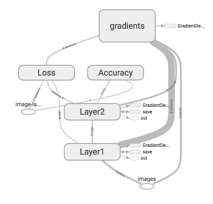
The “Graphs”-tab shows a visualization of the TensorFlow graph we have defined. You can interactively rearrange it until you’re satisfied with how it looks. I think the following image shows the structure of our network pretty well.
In the “Distribution”- and “Histograms”-tabs you can explore the results of the tf.histogram_summary operation we attached to logits, but I won’t go into further details here. More info can be found in the relevant section of the offical TensorFlow documentation.
Further Improvements
Maybe you’re thinking that training the softmax classifier took a lot less computation time than training the neural network. While that’s true, even if we kept training the softmax classifier as long as it took the neural network to train, it wouldn’t reach the same performance. The longer you train a model, the smaller the additional gains get and after a certain point the performance improvement is miniscule. We’ve reached this point with the neural network too. Additional training time would not improve the accuracy significantly anymore. There’s something else we could do though:
The default parameter values are chosen to be pretty ok, but there is some room for improvement left. By varying parameters such as the number of neurons in the hidden layer or the learning rate, we should be able to improve the model’s accuracy some more. A testing accuracy greater than 50% should definitely be possible with this model with some further optimization. Although I would be very surprised if this model could be tuned to reach 65% or more. But there’s another type of network architecture for which such an accuracy is easily doable: convolutional neural networks. These are a class of neural networks which are not fully connected. Instead they try to make sense of local features in their input, which is very useful for analyzing images. It intuitively makes a lot of sense to take spatial information into account when looking at images. In part 3 of this series we will see the principles of how convolutional neural networks work and build one ourselves.
Stay tuned for part 3 on convolutional neural networks and thanks a lot for reading! I’m happy about any feedback you might have!
aYou can also check out other articles I’ve written on my blog.