by Bharath Raj

How to play Quidditch using the TensorFlow Object Detection API

Deep Learning never ceases to amaze me. It has had a profound impact on several domains, beating benchmarks left and right.

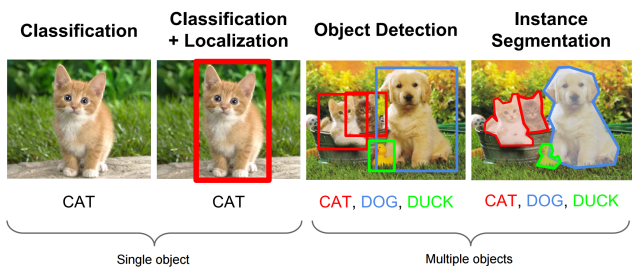
Image classification using convolutional neural networks (CNNs) is fairly easy today, especially with the advent of powerful front-end wrappers such as Keras with a TensorFlow back-end. But what if you want to identify more than one object in an image?

This problem is called “object localization and detection.” It is much more difficult than simple classification. In fact, until 2015, image localization using CNNs was very slow and inefficient. Check out this blog post by Dhruv to read about the history of object detection in Deep Learning, if you’re interested.

Sounds cool. But is it hard to code?

Worry not, TensorFlow’s Object Detection API comes to the rescue! They have done most of the heavy lifting for you. All you need to do is to prepare the dataset and set some configurations. You can train your model and use then it for inference.

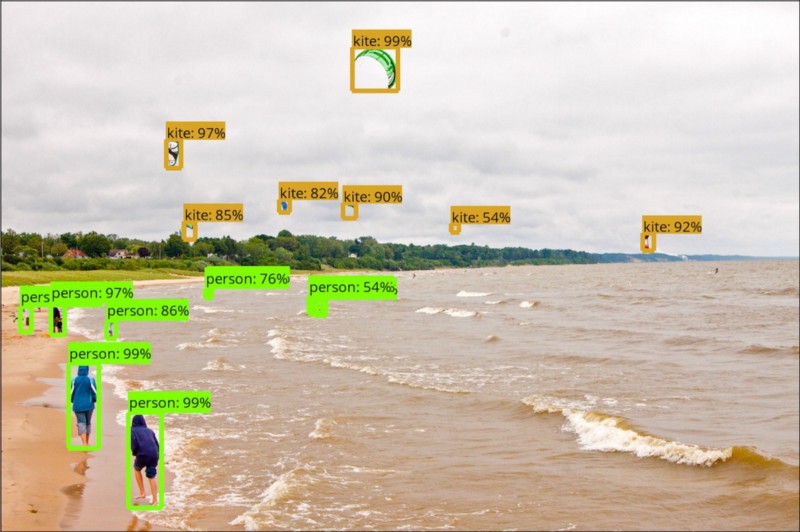
TensorFlow also provides pre-trained models, trained on the MS COCO, Kitti, or the Open Images datasets. You could use them as such, if you just want to use it for standard object detection. The drawback is that, they are pre-defined. It can only predict the classes defined by the datasets.

But, what if you wanted to detect something that’s not on the possible list of classes? That’s the purpose of this blog post. I will guide you through creating your own custom object detection program, using a fun example of Quidditch from the Harry Potter universe! (For all you Star Wars fans, here’s a similar blog post that you might like).

Getting started

Start by cloning my GitHub repository, found here. This will be your base directory. All the files referenced in this blog post are available in the repository.

Alternatively, you can clone the TensorFlow models repo. If you choose the latter, you only need the folders named “slim” and “object_detection,” so feel free to remove the rest. Don’t rename anything inside these folders (unless you’re sure it won’t mess with the code).

Dependencies

Assuming you have TensorFlow installed, you may need to install a few more dependencies, which you can do by executing the following in the base directory:

pip install -r requirements.txt

The API uses Protobufs to configure and train model parameters. We need to compile the Protobuf libraries before using them. First, you have to install the Protobuf Compiler using the below command:

sudo apt-get install protobuf-compiler

Now, you can compile the Protobuf libraries using the following command:

protoc object_detection/protos/*.proto --python_out=.

You need to append the path of your base directory, as well as your slim directory to your Python path variable. Note that you have to complete this step every time you open a new terminal. You can do so by executing the below command. Alternatively, you can add it to your ~/.bashrc file to automate the process.

export PYTHONPATH=$PYTHONPATH:`pwd`:`pwd`/slim

Preparing the inputs

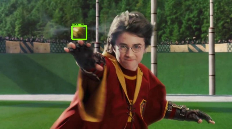
My motive was pretty straightforward. I wanted to build a Quidditch Seeker using TensorFlow. Specifically, I wanted to write a program to locate the snitch at every frame.

But then, I decided to up the stakes. How about trying to identify all the moving pieces of equipment used in Quidditch?

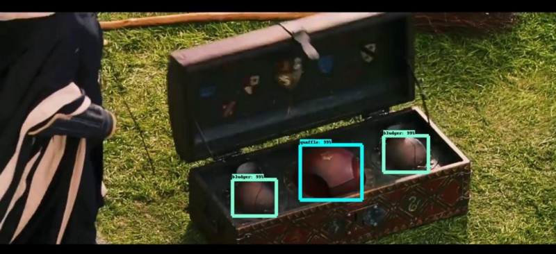
We start by preparing the label_map.pbtxt file. This would contain all the target label names as well as an ID number for each label. Note that the label ID should start from 1. Here’s the content of the file that I used for my project.

item { id: 1 name: ‘snitch’}

item { id: 2 name: ‘quaffle’}

item { id: 3 name: ‘bludger’}

Now, its time to collect the dataset.

Fun! Or boring, depending on your taste, but it’s a mundane task all the same.

I collected the dataset by sampling all the frames from a Harry Potter video clip, using a small code snippet I wrote, using the OpenCV framework. Once that was done, I used another code snippet to randomly sample 300 images from the dataset. The code snippets are available in utils.py in my GitHub repo if you would like to do the same.

You heard me right. Only 300 images. Yeah, my dataset wasn’t huge. That’s mainly because I can’t afford to annotate a lot of images. If you want, you can opt for paid services like Amazon Mechanical Turk to annotate your images.

Annotations

Every image localization task requires ground truth annotations. The annotations used here are XML files with 4 coordinates representing the location of the bounding box surrounding an object, and its label. We use the Pascal VOC format. A sample annotation would look like this:

<annotation>  <filename>182.jpg</filename>  <size>    <width>1280</width>    <height>586</height>    <depth>3</depth>  </size>  <segmented>0</segmented>  <object>    <name>bludger</name>    <bndbox>      <xmin>581</xmin>      <ymin>106</ymin>      <xmax>618</xmax>      <ymax>142</ymax>    </bndbox>  </object>  <object>    <name>quaffle</name>    <bndbox>      <xmin>127</xmin>      <ymin>406</ymin>      <xmax>239</xmax>      <ymax>526</ymax>    </bndbox>  </object></annotation>

You might be thinking, “Do I really need to go through the pain of manually typing in annotations in XML files?” Absolutely not! There are tools which let you use a GUI to draw boxes over objects and annotate them. Fun! LabelImg is an excellent tool for Linux/Windows users. Alternatively, RectLabel is a good choice for Mac users.

A few footnotes before you start collecting your dataset:

• Do not rename you image files after you annotate them. The code tries to look up an image using the file name specified inside your XML file (Which LabelImg automatically fills in with the image file name). Also, make sure your image and XML files have the same name.
• Make sure you resize the images to the desired size before you start annotating them. If you do so later on, the annotations will not make sense, and you will have to scale the annotation values inside the XMLs.
• LabelImg may output some extra elements to the XML file (Such as <pose>, <truncated>, <path>). You do not need to remove those as they won’t interfere with the code.

In case you messed up anything, the utils.py file has some utility functions that can help you out. If you just want to give Quidditch a shot, you could download my annotated dataset instead. Both are available in my GitHub repository.

Lastly, create a text file named trainval. It should contain the names of all your image/XML files. For instance, if you have img1.jpg, img2.jpg and img1.xml, img2.xml in your dataset, you trainval.txt file should look like this:

img1img2

Separate your dataset into two folders, namely images and annotations. Place the label_map.pbtxt and trainval.txt inside your annotations folder. Create a folder named xmls inside the annotations folder and place all your XMLs inside that. Your directory hierarchy should look something like this:

-base_directory|-images|-annotations||-xmls||-label_map.pbtxt||-trainval.txt

The API accepts inputs in the TFRecords file format. Worry not, you can easily convert your current dataset into the required format with the help of a small utility function. Use the create_tf_record.py file provided in my repo to convert your dataset into TFRecords. You should execute the following command in your base directory:

python create_tf_record.py \    --data_dir=`pwd` \    --output_dir=`pwd`

You will find two files, train.record and val.record, after the program finishes its execution. The standard dataset split is 70% for training and 30% for validation. You can change the split fraction in the main() function of the file if needed.

Training the model

Whew, that was a rather long process to get things ready. The end is almost near. We need to select a localization model to train. Problem is, there are so many options to choose from. Each vary in performance in terms of speed or accuracy. You have to choose the right model for the right job. If you wish to learn more about the trade-off, this paper is a good read.

In short, SSDs are fast but may fail to detect smaller objects with decent accuracy, whereas Faster RCNNs are relatively slower and larger, but have better accuracy.

The TensorFlow Object Detection API has provided us with a bunch of pre-trained models. It is highly recommended to initialize training using a pre-trained model. It can heavily reduce the training time.

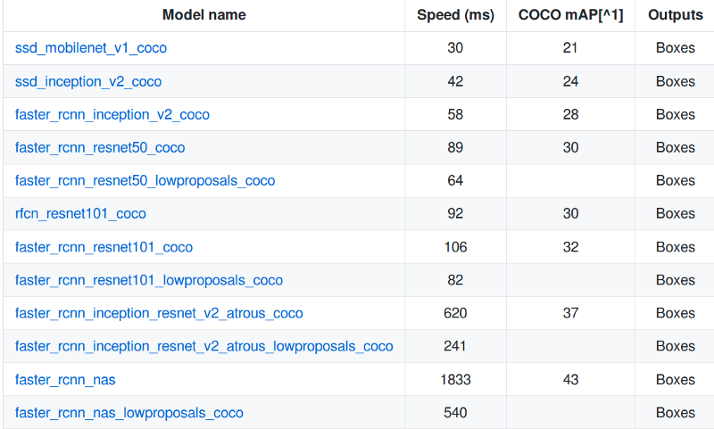
Download one of these models, and extract the contents into your base directory. Since I was more focused on the accuracy, but also wanted a reasonable execution time, I chose the ResNet-50 version of the Faster RCNN model. After extraction, you will receive the model checkpoints, a frozen inference graph, and a pipeline.config file.

One last thing remains! You have to define the “training job” in the pipeline.config file. Place the file in the base directory. What really matters is the last few lines of the file — you only need to set the highlighted values to your respective file locations.

gradient_clipping_by_norm: 10.0  fine_tune_checkpoint: "model.ckpt"  from_detection_checkpoint: true  num_steps: 200000}train_input_reader {  label_map_path: "annotations/label_map.pbtxt"  tf_record_input_reader {    input_path: "train.record"  }}eval_config {  num_examples: 8000  max_evals: 10  use_moving_averages: false}eval_input_reader {  label_map_path: "annotations/label_map.pbtxt"  shuffle: false  num_epochs: 1  num_readers: 1  tf_record_input_reader {    input_path: "val.record"  }}

If you have experience in setting the best hyper parameters for your model, you may do so. The creators have given some rather brief guidelines here.

You’re all set to train your model now! Execute the below command to start the training job.

python object_detection/train.py \--logtostderr \--pipeline_config_path=pipeline.config \--train_dir=train

My Laptop GPU couldn’t handle the model size (Nvidia 950M, 2GB) so I had to run it on the CPU instead. It took around 7–13 seconds per step on my device. After about 10,000 excruciating steps, the model achieved a pretty good accuracy. I stopped training after it reached 20,000 steps, solely because it had taken two days already.

You can resume training from a checkpoint by modifying the “fine_tune_checkpoint” attribute from model.ckpt to model.ckpt-xxxx, where xxxx represents the global step number of the saved checkpoint.

Exporting the model for inference

What’s the point of training the model if you can’t use it for object detection? API to the rescue again! But there’s a catch. Their inference module requires a frozen graph model as an input. Not to worry though: using the following command, you can export your trained model to a frozen graph model.

python object_detection/export_inference_graph.py \--input_type=image_tensor \--pipeline_config_path=pipeline.config \--trained_checkpoint_prefix=train/model.ckpt-xxxxx \--output_directory=output

Neat! You will obtain a file named frozen_inference_graph.pb, along with a bunch of checkpoint files.

You can find a file named inference.py in my GitHub repo. You can use it to test or run your object detection module. The code is pretty self explanatory, and is similar to the Object Detection Demo, presented by the creators. You can execute it by typing in the following command:

python object_detection/inference.py \--input_dir={PATH} \--output_dir={PATH} \--label_map={PATH} \--frozen_graph={PATH} \--num_output_classes={NUM}

Replace the highlighted characters {PATH} with the filename or path of the respective file/directory. Replace {NUM} with the number of objects you have defined for your model to detect (In my case, 3).

Results

Check out these videos to see its performance for yourself! The first video demonstrates the model’s capability to distinguish all three objects, whereas the second video flaunts its prowess as a seeker.

Pretty impressive I would say! It does have an issue with distinguishing heads from Quidditch objects. But considering the size of our dataset, the performance is pretty good.

Training it for too long led to massive over-fitting (it was no longer size invariant), even though it reduced some mistakes. You can overcome this by having a larger dataset.

Thank you for reading this article! Hit that clap button if you did! Hope it helped you create your own Object Detection program. If you have any questions, you can hit me up on LinkedIn or send me an email (bharathrajn98@gmail.com).