

Introduction
I’ve been wanting to write about this topic for a while now. I recently had the opportunity to work on simulating the GoalSeek functionality of Excel for a web application. I found the whole purpose of GoalSeek and how it works fascinating.
The whole purpose of GoalSeek in Excel is finding an input for an equation that will provide the desired solution. To understand how this is supposed to work, we’ll consider something really simple.
What Is Goalseek?
Let’s take the example of finding the amount due based on a principal using the Simple Interest formula.
The equation for the simple interest formula is, well, simple:
A = P(1+rt), eqn(1)P -> principalr -> rate of interestt -> time in yearsWe’ll set the following values:
P -> 10000r -> 7.5t -> 15This gives us the amount due as being:
A = 10000(1+7.5*15) = 1135000Now, let’s say the requirement for our solution changed. Now, instead of finding the amount due based on the principal, rate of interest, and time, we instead need to find the rate of interest that will give us the desired amount due but keeping the principal and time the same.
Let’s alter the example now:
P -> 10000r -> ?t -> 15A -> 1120000Here, we are trying to find the interest rate that will allow us to pay 1120000 instead of 1135000. We can solve this by switching the variables around.
A = P(1+rt) => 1120000 = 10000(1+r*15)1+15*r = 1120000 / 10000 => r = (112 - 1) / 15r = 7.4%Brilliant! There we have it! We did something Excel’s Goalseek does.

One problem, though. That was a really simple equation and problem. What happens if the equation is significantly more complex and involves trigonometric functions along with multiple possible solutions? I’ll give you an example of an equation that you would be able to solve with Goalseek:
f(x, y) = 1550 - (4*x/y * sinh(y/2 * 1500 / (2*x))), eqn(2)Yeah, that definitely looks like a handful. One of the daunting factors when looking at something like this for me is that things are being expressed as functions with dependent variables.
Wasn’t this A = P(1+rt) easier to look at? Granted, part of that is also the fact that the equation is a lot smaller.
But, what if we re-wrote it like this:
f(P, r, t) = P(1+rt)See? It’s still the same thing.
Let’s go back to eqn(2). What if we have the following problem statement:
0 = 1550 - (4*x/0.022 * sinh(0.022/2 * 1500 / (2*x))),solve for xWell, again, all you’re really doing is solving for a variable, but just look at how much harder the problem’s gotten. And it’s primarily because of that pesky sinh sitting in the equation.
Okay, if you’re new to this, I imagine things are getting a little overwhelming. Let’s take a step back and think about what we’ve figured out so far.
- We figured out that there’s no real difference between writing a function with notations like the following two:
f(P, r, t) = P(1+rt)A = P(1+rt)2. We figured out that we can solve for one variable to give us the desired result. However, the more complex the equation is, the more complicated getting the solution is.
We have two equations of very opposing difficulties to solve. I will introduce a third equation that will help to bridge the gap
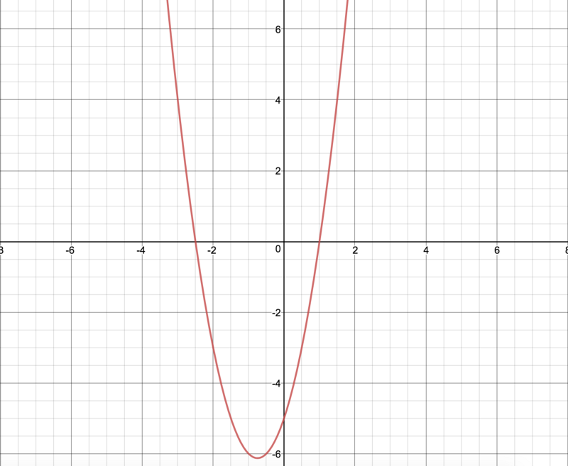
y = 2x^2+3x-5, eqn(3)The equation above is a basic parabolic function. This is what the equation looks like when plotted.
Okay, now let’s think about how to solve this equation. Let’s say we want to solve for x so that y = 0:
y = 2x^2+3x-5 => 2x^2+3x-5 = 0x = [-3 + sqrt(3^2 - 4*2*(-5))] / (2*2), [-3 - sqrt(3^2 - 4*2*(-5))] / (2*2)]x = 1, -2.5If you are wondering where I got the equation for the solutions from, notice it’s just the classic solution to a quadratic equation.
y = ax^2+bx+c, where y = 0 => ax^2+bx+c = 0x = -b+sqrt(b^2-4ac) / 2a, x = -b-sqrt(b^2-4ac) / 2aNote: If you want to find out how this solution was derived, take a look here.
Well, that’s one way to solve the equation. You could potentially write a parser that could accept any equation, check the coefficients, accurately separate them and then attempt to solve the equation. You could also use the wonderful algebra.js library here, which does what I just described.
However, if you look at the graph, you will notice that you could have solved this graphically. The goal was to find the point on the curve where y = 0
Well, look carefully and see where the curve crosses the X-axis. It crosses it at two points: [1, -2.5] There’s your solution!
Now, you’re probably thinking that’s all great, but I can’t exactly teach a computer to look at the graph, find the points where it crosses the X-axis and identify those points. Well, potentially you could, with some form of model trained for image recognition, but that’s another post. So, how do we find our way around this?
There are two methods we can use, and these are the ones I will be exploring in depth in this article.
They are called the Newton-Raphson method and the bisection method.
I’ll give you a brief overview of how each method works.
TL;DR Version
The Newton-Raphson method works by picking a random point and drawing a tangent line at that point. It then calculates a new x value which is closer to the root. If you keep repeating this, you will find the root.
The Bisection method works on the principle of finding the interval within which the root lies. Once the accurate interval lies, the solution is found by using an algorithm similar to the one used for binary search.
Let’s get into each one in more detail.
Newton-Raphson Method
Okay, let’s dig into the Newton-Raphson method. The Newton-Raphson method is based on three major ideas.
- The tangent to a curve at a specific point is a straight line
- The tangent to a curve at a specific point is also the derivative of the curve at that point
- The equation of a straight line, which is:
y = mx + c

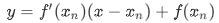
The image above is that of a random curve with a tangent drawn to it.
We’ve picked a random point x_n on the X-axis.
f(x_n) is the equivalent of the point on the curve. i.e the y-intercept
f’(x_n) is the tangent to the curve at the point f(x_n).
x_(n+1) is the point where the tangent intercepts the X-axis.
Remember, we said we wanted to find the point where the curve crosses the X-axis, as this would give us our solution. Notice, the point x_(n+1) is a lot closer to the solution than x_n was, despite us picking x_n at random.
Well, what if we repeated the same process, except this time with x_(n+1) as our new point initial point? Well, presumably we would end up with a new x that is even closer to the solution.
So, how do we find the point x_(n+1)given the equation, the derivative and the original x_n?
Let’s go back to the equation of a straight line: y = mx+c
We said that the tangent to a curve at a point is a straight line.
We also said that the y-intercept is equal to f(x_n)
We know from calculus, that the derivative is equal to the slope.
Therefore, we get the following:
Now, we need to find the root of this tangent line, so set y = 0 and x = x_(n+1), and solve for x_(n+1)
This gives us the following:
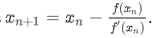
Now, we have everything we need to solve for x_(n+1).
This went way over my head the first time I saw all the equations, so let’s try it with an example to see how it works.
We’ll take eqn(2) and work through that. Let’s pick x_n=3
f(x) = 2x^2+3x-5f'(x) = 4x+3f(3) = 18+9-5 = 22f'(3) = 15x_1 = 3 - 22/15 = 1.53f(1.53) = 4.2718f'(1.53) = 9.12x_2 = 1.53 - 4.2718/9.12 = 1.0616If you follow that all the way through, you should get a solution where x=1 and as we know from the earlier graph, this is one of our solutions.
If you notice what we did above was just follow a series of steps in a certain order repeatedly, i.e. the very definition of an algorithm. Here is what the code looks like for the same.
The code snippet makes heavy use of the math.js library. The main functions I am making use of are the math.derivative and the math.eval functions. Respectively, they calculate the derivative of an expression and evaluate an expression based on an object of key-value pairs.
The bit of the code snippet I want to draw your attention to is lines 14–16.
if (Math.abs(result - guess) < Math.exp(-15)) { return result }What we’re doing here is defining the base condition to end our iteration. We’re saying that if the difference between x_n and x_(n+1) is less than 10^(-15) return the result.
If you work through the prior exercise all the way through, you’ll arrive at a situation where each successive x value is almost identical to the prior x value, and this is how we know we have found a solution.
I have a nice little simulation built with d3.js in codepen showing you how this would run iteratively.
Just enter a value in the input box and hit submit and you can watch the algorithm run graphically.
Note: Please try a range of sensible inputs, I haven’t exactly built a robust system here.
Bisection Method
Okay, so we figured out how the Newton-Raphson method works. Let’s tackle the bisection method next.
The bisection method is a lot easier to understand than the Newton-Raphson method. It’s based on a very simple mathematical property:
If a function f(x) is continuous on the interval [a, b] and the sign of f(a) !== f(b), then there is a value c in the range (a, b) where f(c) = 0. In other words, c is the root of the equation.
If that didn’t make sense to you, think about it purely numerically and then purely graphically.
Let’s say you have the following interval: [-7, 6]. Now if I ask you to count just the integers from -7 to 6, you would also count 0 at some point in that interval. That’s essentially what the property above says.
Let’s look at what this means graphically.
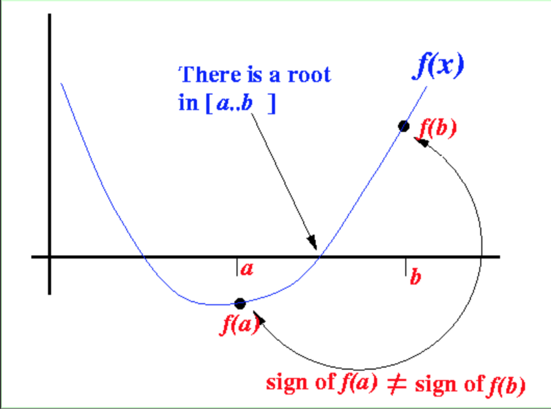
The above function is a continuous line and it goes from negative to positive, which implies that it has to cross 0 at some point. Since it has to cross 0, that means the root lies in this interval.
Okay, this means that using the bisection method is a two-step process.
- Find the interval within which the root lies, if such an interval exists
- Find the actual root within this interval
Here’s the code for how you’d find the interval:
Again, I am making use of mathjs here, so you can look up the documentation for that.
The interesting bit of this algorithm is in lines 18–26, where I am making a check to see if either my function evaluation of the left interval or right interval has resulted in something that is NaN . I will explain why I included this code block when we explore how to solve eqn(2).
Once we have the interval within which the solution lies, we can turn our attention to actually finding the solution itself.
If you’ve ever tried to write a binary search algorithm on an array, the code snippet above should look very familiar to you. We are employing more or less the same approach here. Here are the steps involved.
- I start with my left and right intervals and find a mid-point
- Check whether the solution lies to the left of the mid-point or to the right of the mid-point
- If it lies to the left, set
right = mid, else setleft = mid
Eventually, the midpoint will be the root itself.
Here is a little simulation running through what is actually going on.
Note: I apologise for how ugly the simulation looks, unfortunately styling is not my forte. Again, sensible range of inputs, because otherwise its going take quite a while for the simulation to run.
In the pen above, enter a value, and the simulation will attempt to find an interval within which a potential root could exist. Once it has found an interval, it will start trying to find the root by using the algorithm we discussed immediately prior to this.
Solving Complex Equations
Alright, we’ve explored two different methods of finding the roots of equations. Now, its time to explore the more complex eqn(2) we had and see which of these methods can solve that equation.
I’ll put the equation below so it’s clear
f(x, y) = 1550 - (4*x/y * sinh(y/2 * 1500 / (2*x))), eqn(2)Solve for f(x, y) = 0, where y = 0.0220 = 1550 - (4*x/0.022 * sinh(0.022/2 * 1500 / (2*x)))First, let’s visualize what this equation looks like. It’ll give us a much better intuition for why something might go wrong.
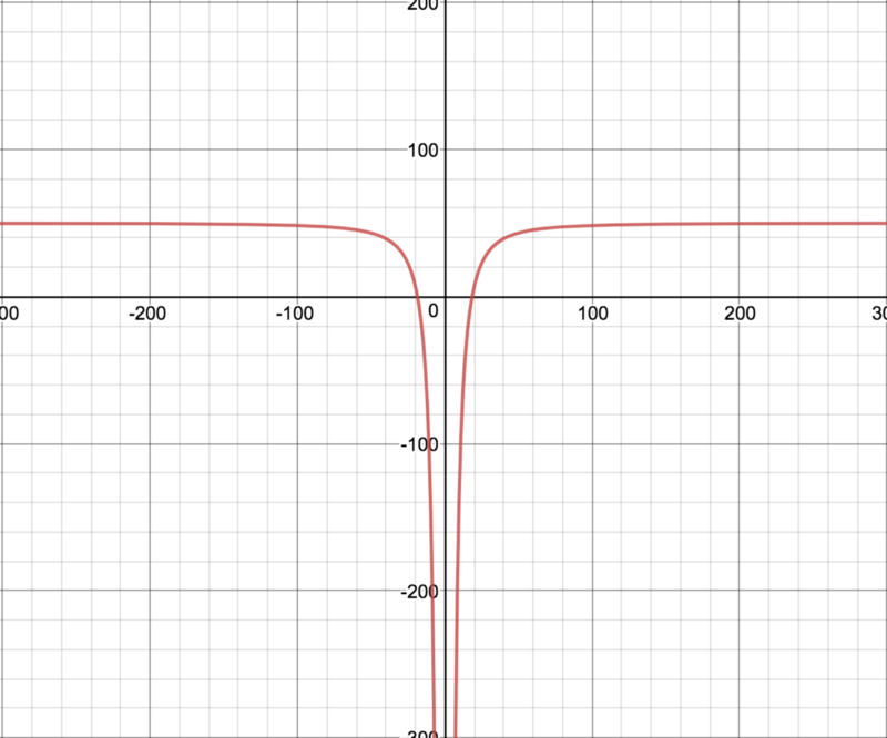
The thing to note about this equation is that it tends to infinity as x tends to 0. This is going to pose a problem for the Newton-Raphson method because the Newton-Raphson solution tends to follow the path of the tangent, in which case it might quickly dissolve to infinity as a solution unless it managed to hit on the solution by chance.
Try running the above equation with the Newton-Raphson method and you’ll see what I mean. You will probably get a result of null.
The bisection method, on the other hand, will work quite nicely for this. It works well because we are taking very small incremental steps with a step size we have control over. Run the below codepen and you should see how nicely the bisection method works for most equations.
The code above is almost identical to the previous version we set up for the bisection method, baring a few differences. I set up a separate codepen so I could be spared the effort of having to allow a way to enter equations, which would require extensive checks and error handling. Also, this equation requires special boundaries for defining its data since it tends to infinity as x approaches 0. If you’re interested you can see what I mean if you have a look through the code.
Now, in the bisection method code I told you about this block of code here:
if (Number.isNaN(result_left)) { left -= stepSize scope_left[variable] = left result_left = math.eval(eqn, scope_left) } if (Number.isNaN(result_right)) { right += stepSize scope_right[variable] = right result_right = math.eval(eqn, scope_right)}So the reason I have this is to handle situations like those that arise for eqn(2). Because eqn(2) tends to infinity as x tends to 0, there could be a situation where the evaluation of the equation returns either NaN or Infinity . To avoid this situation, I simply shift the equation over by the step size repeatedly until I can get back to the domain of the function that lies in the real number range.
Bisection > Newton-Raphson?
This brings me to an important point, why did Newton-Raphson fail for this equation? We know that since Newton-Raphson follows the tangent of the curve at different points, it can dissolve to infinity if the equation tends to infinity at any particular point. This highlights one of the shortcomings of the Newton-Raphson method.
- The Newton-Raphson method works well for a continuous function. If the function is discontinuous as in eqn(2) is, it will typically fail.
- Newton-Raphson cannot account for multiple maxima and minima in a function.
Take the following graph for example.
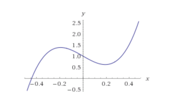
Pick a point at random between -0.19 and +0.19, and you should see that you will get a negative slope, which means the tangent to the curve at that point will intercept the X-axis at a point further away from the root, which goes against the principle of the Newton-Raphson method. This implies that Newton-Raphson will typically fail for cubic and higher order equations.
The Bisection Method should not have the same problem because it depends on finding an interval within which the solution has to lie, and curves like the above will not be an obstacle to that as long it is continuous in that domain.
If you compare the two in terms of Big(O) notation, it seems obvious that Newton-Raphson runs on fewer iterations than the Bisection method, simply because it converges much faster when you view it graphically. Ironically, if you run this with a timing process, it frequently turns out that, given the same starting point, the Bisection method runs faster than the Newton-Raphson method.
This is because the Newton-Raphson involves computing a derivative at every step, which turns out to be very computationally expensive. Incrementing and decrementing a number on the other is relatively computationally inexpensive.
If you want to run the same on your machine and check the results, check out the repo here. You can clone that repo, run npm install and then npm run start on your machine, and you should see the results of running both the Newton-Raphson and Bisection method on an identical equation given the same initial guess.
Conclusion
Okay, we’ve covered a lot here. But honestly, this is such a ridiculously vast topic that I’ve barely scratched the surface. Convergence of equations is a widely studied topic. Consider one of the most basic things we haven’t covered: finding multiple roots.
You can of course modify the algorithms provided in this article to achieve that.
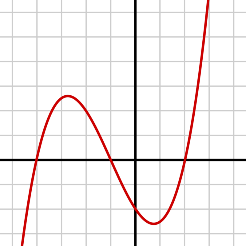
Take the equation below, for example. It has 3 roots (3 points where it intercepts the X-axis, and you need to find all of these roots).
I’m going to post all my sources here, feel free to look through them.
Note: If you have questions or comments about the article, don’t hesitate to reach out to me via comments on this article or on GitHub or Twitter.