
Relational databases handle data smoothly, whether working with small volumes or processing millions of rows. We will be looking at how we can use relational databases according to our needs, and get the most out of them.
MySQL has been a popular choice for small to large enterprise companies because of its ability to scale. Similarly, PostgreSQL has also seen a rise in popularity.
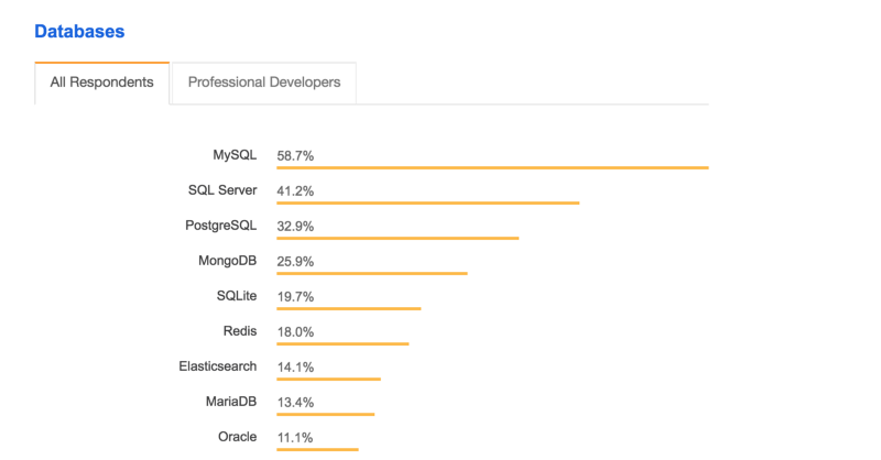
According to the Stack Overflow survey 2018, MySQL is the most popular database among all users.
The examples described below are using InnoDB as MySQL engine. These are not limited only to MySQL but are also relevant with other relational databases like PostgreSQL. All the benchmarking is done on a machine with 8GB RAM and with an i5 2.7 GHz processor.
Let’s get started with the basics of how relational database store the data.
Understanding Relational Databases
Storage
MySQL is a relational database where all data is represented in terms of tuples, grouped into relations. A tuple is represented by its attributes.

Let’s say we have an application where people can loan books. We will need to store all the book lending transactions. In order to store them, we have designed a simple relational table with the following command:
> CREATE TABLE book_transactions ( id INTEGER NOT NULL AUTO_INCREMENT, book_id INTEGER, borrower_id INTEGER, lender_id INTEGER, return_date DATE, PRIMARY KEY (id));The table looks like:
book_transactions
------------------------------------------------
id  borrower_id  lender_id  book_id  return_date
Here id is the primary key and borrower_id, lender_id, book_id are the foreign keys. After we launch our application there are few transactions recorded:
book_transactions
------------------------------------------------
id  borrower_id  lender_id  book_id  return_date
------------------------------------------------
1   1            1          1        2018-01-13
2   2            3          2        2018-01-13
3   1            2          1        2018-01-13
Fetching the data
We have a dashboard page for each user where they can see the transactions of their books rented. So let’s fetch the book transactions for a user:
> SELECT * FROM book_transactions WHERE borrower_id = 1;
book_transactions
------------------------------------------------
id  borrower_id  lender_id  book_id  return_date
------------------------------------------------
1   1            1          1        2018-01-13
2   1            2          1        2018-01-13
This scans the relation sequentially and gives us the data for the user. This seems to be very fast, as there are very few data in our relation. To see the exact time of the query execution, set profiling to be true by executing the following command:
> set profiling=1;Once the profiling is set, run the query again and use the following command to look into the execution time:
> show profiles;This will return the duration of the query we executed.
Query_ID | Duration   | Query
       1 | 0.00254000 | SELECT * FROM book_transactions ...
The execution seems to be very good.
Slowly, the book_transactions table starts to get filled with data, as there are a lots of transactions going on.
The problem
This increases the number of tuples in our relation. With this, the time it takes to fetch the book transactions for the user will start to take more time. MySQL needs to go through all the tuples to find the result.
To insert a lot of data into this table, I wrote the following stored procedure:
DELIMITER //
 CREATE PROCEDURE InsertALot()
   BEGIN
   DECLARE i INT DEFAULT 1;
   WHILE (i <= 100000) DO
    INSERT INTO book_transactions (borrower_id, lender_id, book_id,   return_date) VALUES ((FLOOR(1 + RAND() * 60)), (FLOOR(1 + RAND() * 60)), (FLOOR(1 + RAND() * 60)), CURDATE());
    SET i = i+1;
   END WHILE;
 END //
 DELIMITER ;
* It took around 7 minutes to insert 1.5 million data
This inserts 100,000 random records in our table book_transactions. After running this, the profiler shows a slight increase in the runtime:
Query_ID | Duration   | Query
       1 | 0.07151000 | SELECT * FROM book_transactions ...
Let’s add few more data running the above procedure and see what happens. With more and more data added, the duration of the query increases. With 1.5 million data inserted into the table, the response time to get the same query is now increased.
Query_ID | Duration   | Query
       1 | 0.36795200 | SELECT * FROM book_transactions ...
This is just a simple query involving an integer field.
With more compound queries, order queries, and count queries, the execution time gets even worse.
This does not seem to be a long time for a single query, but when we have thousands or even millions of queries running every minute, this makes a big difference.
There will be lot more wait time and this will hamper the overall performance of the application. The execution time for the same query increased from 2ms to 370ms.
Getting the speed back
Index
MySQL and other databases provide indexing, a data structure that helps to retrieve data faster.
There are different types of indexing in MySQL:
- Primary Key — Index added to the primary key. By default, primary keys are always indexed. It also ensures that the two rows do not have the same primary key value.
- Unique — Unique key index insures that no two rows in a relation have the same value. Multiple Null values can be stored with a unique index.
- Index — Addition to any other fields other than the primary key.
- Full Text — Full text index helps queries against character-based data.
There are mostly two ways an index is stored:
Hash — this is mostly used for exact matching (=), and does not work with comparisons(≥, ≤)
B-Tree — This is the mostly common way in which the above mentioned index types are stored.
MySQL uses a B-Tree as its default indexing format. The data are stored in a binary tree which makes the retrieval of data fast.
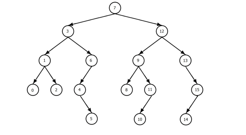
The data organization done by the B-tree helps to skip the full table scan across all tuples in our relation.
There are a total of 16 nodes in the above B-Tree. Let’s say we need to find the number 6. We only need to do a total number of 3 scans to get the number. This helps improve the performance of search.
So to improve the performance on our book_transactions relation, let’s add the index on the field lender_id.
> CREATE INDEX lenderId ON book_transactions(lender_id)
----------------------------------------------------
* It took around 6.18sec Adding this index
The above command adds an index on the lender_id field. Let’s look at how this affects performance for the 1.5 million data that we have by running the same query again.
> SELECT * FROM book_transactions WHERE lender_id = 1;
Query_ID | Duration   | Query
       1 | 0.00787600 | SELECT * FROM book_transactions ...
Woohoo! We are back now.
It is as fast as it used to be when there were only 3 records in our relation. With the right index added, we can see a dramatic improvement in performance.
Composite and single index
The index we added was a single field index. Indices can also be added to a composite field.
If our query involved multiple fields, a composite index would have helped us. We can add a composite index with the following command:
> CREATE INDEX lenderReturnDate ON book_transactions(lender_id, return_date);Other Usage of Indices
Querying is not the only use of indices. They can be used for the ORDER BY clause as well. Let’s order the records with respect to lender_id.
> SELECT * FROM book_transactions ORDER BY lender_id;
1517185 rows in set (4.08 sec)
4.08 sec, that’s a lot! So what went wrong? We have our index in place. Let’s deep dive into how the query is being executed with the help of EXPLAIN clause.
Using Explain
We can add an explain clause to see how the query will be executed in our current dataset.
> EXPLAIN SELECT * FROM book_transactions ORDER BY lender_id;
The output of this is as shown bellow:
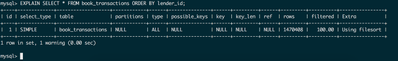
There are various fields that explain returns. Let’s look into the table above and find out the problem.
rows: Total number of rows that will be scanned
filtered: The percentage of row that will be scanned to get the data
type: It’s given if the index is being used. ALL means it is not using index
possible_keys, key, key_len are all NULL, which means that no index is being used.
So why is the query not using index?
This is because we have select * in our query, which means we are selecting all the fields from our relation.
The index only has information about fields that are indexed, and not about other fields. This means MySQL will need to go to the main table to fetch data again.
So how should we write the query?
Select Only the required field
To remove the need to go to the main table for the query, we need to select only the value that is present in the index table. So let’s change the query:
> SELECT lender_id FROM book_transactions ORDER BY lender_id;
This will return the result in 0.46 seconds, which is way faster. But there is still room for improvement.
As this query is done on all the 1.5 million records that we have, it is taking a little more time as it needs to load data into memory.
Use Limit
We might not need all the 1.5 million data at the same time. So instead of fetching all the data, using LIMIT and fetching data in batches is a better way to go.
> SELECT lender_id
  FROM book_transactions
  ORDER BY lender_id LIMIT 1000;
With a limit in place, the response time now improves drastically, and executes in 0.0025 seconds. Now we can fetch next batch with OFFSET.
> SELECT lender_id
  FROM book_transactions
  ORDER BY lender_id LIMIT 1000 OFFSET 1000;
This will fetch the next 1000 row batch. With this we can increase the offset and limit to get all the data. But there is a ‘gotcha’! With an increase in offset, the performance of the query decreases.
This is because MySQL will scan through all the data to reach the offset point. So it is better not to use higher offset.
What about Count query?
InnoDB engine has an ability to write concurrently. This makes it highly scalable and improves the throughput per second.
But this comes at a cost. InnoDB cannot add a cache counter for the number of records in any table. So, the count has to be done in real time by scanning through all the filtered data. This makes the COUNT query slow.
So it is recommended to calculate the summarized count data from application logic for large number of data.
Why not add an index to all fields?
Adding index helps improve performance a lot, but it also comes with a cost. It should be used effectively. Adding an index to more fields has the following issues:
- Needs a lot of memory, bigger machine
- When we delete, there is a re-index (CPU intensive and slower deletes)
- When we add anything, there is reindex (CPU intensive and slower inserts)
- Update does not do full reindex, so update is faster and CPU efficient.
We are now clear that adding an index helps a lot. But we cannot select all the data, except that which is indexed for fast performance.
So how can we select all the attributes and still get fast performance?
Partitioning
While we build indices, we only have information about the field that is indexed. But we do not have data of the fields that are not present in the index.
So, as we said earlier, MySQL needs to look back at the main table to get the data for other fields. This can slow down the execution time.
The way we can solve this is by using partitioning.
Partitioning is a technique in which MySQL splits a table’s data into multiple tables, but still manages it as one.
While doing any kind of operation in the table we need to specify which partition is being used. With data being broken down, MySQL has a smaller data set to query on. Figuring out the right partitioning according to the needs is key for high performance.
But if we are still using the same machine, will it scale?
Sharding
With a huge data set, storing all your data on the same machine can be troublesome.
A specific partition can be heavy and needs more querying, while other are less. So one will affect another. They cannot scale separately.
Let’s say the recent three months worth of data are the most used, where as the older one are less used. Perhaps the recent data are mostly updated/created whereas the old data are mostly only ever read.
To resolve this issue, we can move the recent three months partition to another machine. Sharding is a way in which we divide a big data set into smaller chunks, and move to separate RDBMS. In other words sharding can also be called ‘horizontal partitioning’.
Relational databases have the ability to scale as the application grows. Finding out the right index and tuning the infrastructure according to need is necessary.
Also Posted on Milap Neupane Blog: How to work Optimally with relational Databases