by gk_

Image Recognition Demystified

Nothing in machine learning captivates the imagination quite like the ability to recognize images. Identifying imagery must connote “intelligence,” right? Let’s demystify.

The ability to “see,” when it comes to software, begins with the ability to classify. Classification is pattern matching with data. Images are data in the form of 2-dimensional matrices.

Image recognition is classifying data into one bucket out of many. This is useful work: you can classify an entire image or things within an image.

One of the classic and quite useful applications for image classification is optical character recognition (OCR): going from images of written language to structured text.

This can be done for any alphabet and a wide variety of writing styles.

Steps in the process

We’ll build code to recognize numerical digits in images and show how this works. This will take 3 steps:

1. gather and organize data to work with (85% of the effort)
2. build and test a predictive model (10% of the effort)
3. use the model to recognize images (5% of the effort)

Preparing the data is by far the largest part of our work, this is true of most data science work. There’s a reason it’s called DATA science!

The building of our predictive model and its use in predicting values is all math. We’re using software to iterate through data, to iteratively forge “weights” within mathematical equations, and to work with data structures. The software isn’t “intelligent”, it works mathematical equations to do the narrow knowledge work, in this case: recognizing images of digits.

In practice, most of what people label “AI” is really just software performing knowledge work.

Our predictive model and data

We’ll be using one of the simplest predictive models: the “k-nearest neighbors” or “kNN” regression, first published by E. Fix, J.L. Hodges in 1952.

A simple explanation of this algorithm is here and a video of its math here. And also here for those that want to build the algorithm from scratch.

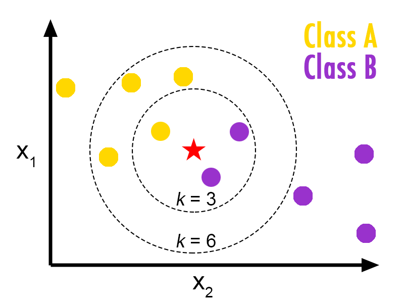
Here’s how it works: imagine a graph of data points and circles capturing k points, with each value of k validated against your data.

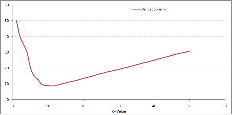
The validation error for k in your data has a minimum which can be determined.

Given the ‘best’ value for k you can classify other points with some measure of precision.

We’ll use scikit learn’s kNN algorithm to avoid building the math ourselves. Conveniently this library will also provides us our images data.

Let’s begin.

The code is here, we’re using iPython notebook which is a productive way of working on data science projects. The code syntax is Python and our example is borrowed from sk-learn.

Start by importing the necessary libraries:

Next we organize our data:

training images: 1527, test images: 269

You can manipulate the fraction and have more or less test data, we’ll see shortly how this impacts our model’s accuracy.

By now you’re probably wondering: how are the digit images organized? They are arrays of values, one for each pixel in an 8x8 image. Let’s inspect one.

# one-dimension[  0.   1.  13.  16.  15.   5.   0.   0.   0.   4.  16.   7.  14.  12.   0.   0.   0.   3.  12.   2.  11.  10.   0.   0.   0.   0.   0.   0.  14.   8.   0.   0.   0.   0.   0.   3.  16.   4.   0.   0.   0.   0.   1.  11.  13.   0.   0.   0.   0.   0.   9.  16.  14.  16.   7.   0.   0.   1.  16.  16.  15.  12.   5.   0.]

# two-dimensions[[  0.   1.  13.  16.  15.   5.   0.   0.] [  0.   4.  16.   7.  14.  12.   0.   0.] [  0.   3.  12.   2.  11.  10.   0.   0.] [  0.   0.   0.   0.  14.   8.   0.   0.] [  0.   0.   0.   3.  16.   4.   0.   0.] [  0.   0.   1.  11.  13.   0.   0.   0.] [  0.   0.   9.  16.  14.  16.   7.   0.] [  0.   1.  16.  16.  15.  12.   5.   0.]]

The same image data is shown as a flat (one-dimensional) array and again as an 8x8 array in an array (two-dimensional). Think of each row of the image as an array of 8 pixels, there are 8 rows. We could ignore the gray-scale (the values) and work with 0’s and 1’s, that would simplify the math a bit.

We can ‘plot’ this to see this array in its ‘pixelated’ form.

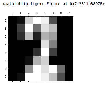
What digit is this? Let’s ask our model, but first we need to build it.

KNN score: 0.951852

Against our test data our nearest-neighbor model had an accuracy score of 95%, not bad. Go back and change the ‘fraction’ value to see how this impacts the score.

array([2])

The model predicts that the array shown above is a ‘2’, which looks correct.

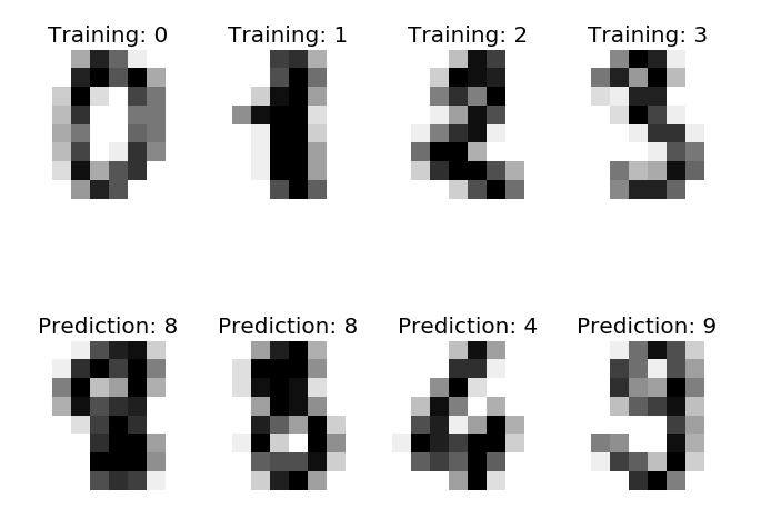
Let’s try a few more, remember these are digits from our test data, we did not use these images to build our model (very important).

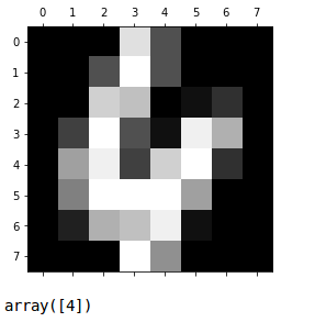
Not bad.

We can create a fictional digit and see what our model thinks about it.

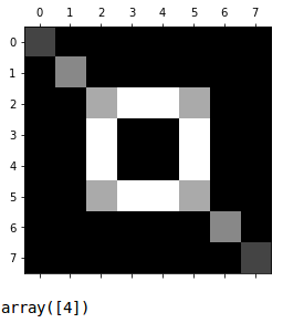
If we had a collection of nonsensical digit images we could add those to our training with a non-numeric label — just another classification.

So how does image recognition work?

• image data is organized: both training and test, with labels (X, y)

Training data is kept separate from test data, which also means we remove duplicates (or near-duplicates) between them.

• a model is built using one of several mathematical models (kNN, logistic regression, convolutional neural network, etc.)

Which type of model you choose depends on your data and the type and complexity of the classification work.

• new data is put into the model to generate a prediction

This is lighting fast: the result of a single mathematical calculation.

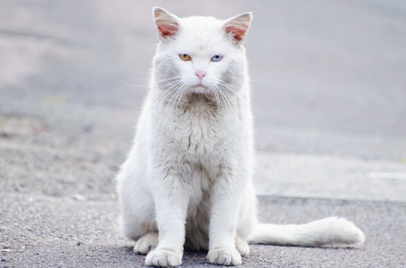
If you have a collection of pictures with and without cats, you can build a model to classify if a picture contains a cat. Notice you need training images that are devoid of any cats for this to work.

Of course you can apply multiple models to a picture and identify several things.

Large Data

A significant challenge in all of this is the size of each image since 8x8 is not a reasonable image size for anything but small digits, it’s not uncommon to be dealing with 500x500 pixel images, or larger. That’s 250,000 pixels per image, so 10,000 images of training means doing math on 2.5Billion values to build a model. And the math isn’t just addition or multiplication: we’re multiplying matrices, multiplying by floating-point weights, calculating derivatives. This is why processing power (and memory) is key in certain machine learning applications.

There are strategies to deal with this image size problem:

• use hardware graphic processor units (GPUs) to speed up the math
• reduce images to smaller dimensions, without losing clarity
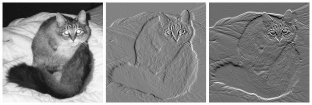
• reduce colors to gray-scale and gradients (you can still see the cat)

• look at sections of an image to find what you’re looking for

The good news is once a model is built, no matter how laborious that was, the prediction is fast. Image processing is used in applications ranging from facial recognition to OCR to self-driving cars.

Now you understand the basics of how this works.