by Shruti Tanwar

Let’s simplify algorithm complexities!

It’s been a while since I started thinking about going back to the basics and brushing up on core computer science concepts. And I figured, before jumping into the pool of heavyweight topics like data structures, operating systems, OOP, databases, and system design (seriously, the list is endless)?, I should probably pick up the topic we all kinda don’t wanna touch: algorithm Complexity Analysis.

Yep! The concept which is overlooked most of the time, because the majority of us developers are thinking, “Hmm, I probably won’t need to know that while I actually code!”.?

Well, I’m not sure if you’ve ever felt the need to understand how algorithm analysis actually works. But if you did, here’s my try at explaining it in the most lucid manner possible. I hope it helps someone like me.?

What is algorithm analysis anyway, and why do we need it??

Before diving into algorithm complexity analysis, let’s first get a brief idea of what algorithm analysis is. Algorithm analysis deals with comparing algorithms based upon the number of computing resources that each algorithm uses.

What we want to achieve by this practice is being able to make an informed decision about which algorithm is a winner in terms of making efficient use of resources(time or memory, depending upon use case). Does this make sense?

Let’s take an example. Suppose we have a function product() which multiplies all the elements of an array, except the element at the current index, and returns the new array. If I am passing [1,2,3,4,5] as an input, I should get [120, 60, 40, 30, 24] as the result.

The above function makes use of two nested for loops to calculate the desired result. In the first pass, it takes the element at the current position. In the second pass, it multiplies that element with each element in the array — except when the element of the first loop matches the current element of the second loop. In that case, it simply multiplies it by 1 to keep the product unmodified.

Are you able to follow? Great!

It’s a simple approach which works well, but can we make it slightly better? Can we modify it in such a way that we don’t have to make two uses of nested loops? Maybe storing the result at each pass and making use of that?

Let’s consider the following method. In this modified version, the principle applied is that for each element, calculate the product of the values on the right, calculate the products of values on the left, and simply multiply those two values. Pretty sweet, isn’t it?

Here, rather than making use of nested loops to calculate values at each run, we use two non-nested loops, which reduces the overall complexity by a factor of O(n) (we shall come to that later).

We can safely infer that the latter algorithm performs better than the former. So far, so good? Perfect!

At this point, we can also take a quick look at the different types of algorithm analysis which exist out there. We do not need to go into the minute level details, but just need to have a basic understanding of the technical jargon.

Depending upon when an algorithm is analyzed, that is, before implementation or after implementation, algorithm analysis can be divided into two stages:

• Apriori Analysis − As the name suggests, in apriori(prior), we do analysis (space and time) of an algorithm prior to running it on a specific system. So fundamentally, this is a theoretical analysis of an algorithm. The efficiency of an algorithm is measured under the assumption that all other factors, for example, processor speed, are constant and have no effect on the implementation.
• Apostiari Analysis − Apostiari analysis of an algorithm is performed only after running it on a physical system. The selected algorithm is implemented using a programming language which is executed on a target computer machine. It directly depends on system configurations and changes from system to system.

In the industry, we rarely perform Apostiari analysis, as software is generally made for anonymous users who might run it on different systems.
Since time and space complexity can vary from system to system, Apriori Analysis is the most practical method for finding algorithm complexities. This is because we only look at the asymptotic variations (we will come to that later) of the algorithm, which gives the complexity based on the input size rather than system configurations.

Now that we have a basic understanding of what algorithm analysis is, we can move forward to our main topic: algorithm complexity. We will be focusing on Apriori Analysis, keeping in mind the scope of this post, so let’s get started.

Deep dive into complexity with asymptotic analysis

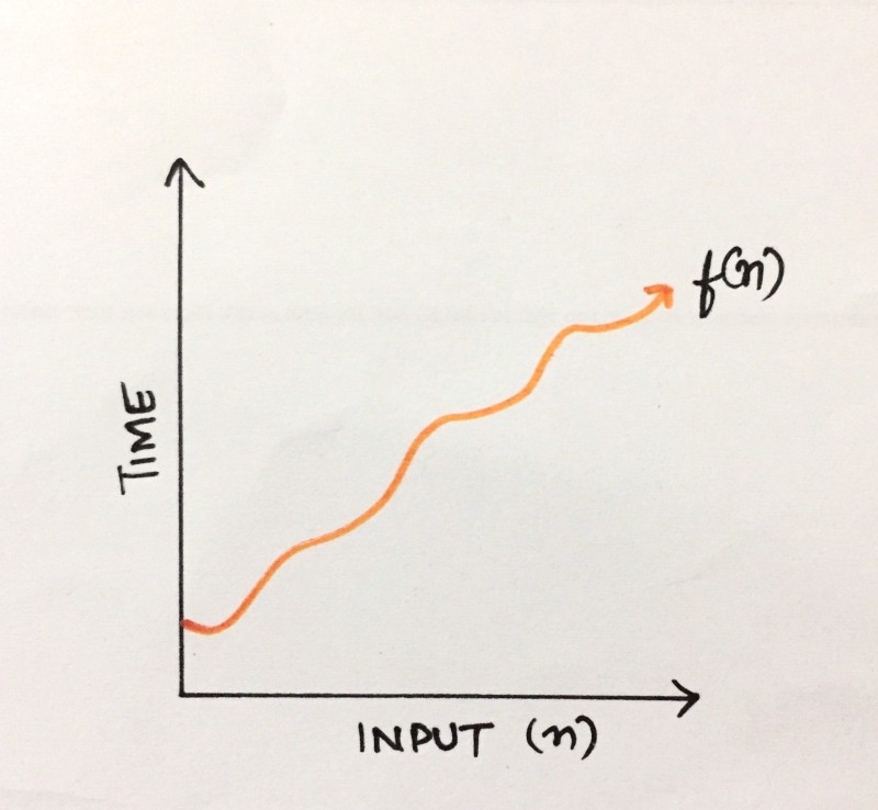
Algorithm complexity analysis is a tool that allows us to explain how an algorithm behaves as the input grows larger.

So, if you want to run an algorithm with a data set of size n, for example, we can define complexity as a numerical function f(n) — time versus the input size n.

Now you must be wondering, isn’t it possible for an algorithm to take different amounts of time on the same inputs, depending on factors like processor speed, instruction set, disk speed, and brand of the compiler? If yes, then pat yourself on the back, cause you are absolutely right!?

This is where Asymptotic Analysis comes into this picture. Here, the concept is to evaluate the performance of an algorithm in terms of input size (without measuring the actual time it takes to run). So basically, we calculate how the time (or space) taken by an algorithm increases as we make the input size infinitely large.

Complexity analysis is performed on two parameters:

1. Time: Time complexity gives an indication as to how long an algorithm takes to complete with respect to the input size. The resource which we are concerned about in this case is CPU (and wall-clock time).
2. Space: Space complexity is similar, but is an indication as to how much memory is “required” to execute the algorithm with respect to the input size. Here, we dealing with system RAM as a resource.

Are you still with me? Good! Now, there are different notations which we use for analyzing complexity through asymptotic analysis. We will go through all of them one by one and understand the fundamentals behind each.

The Big oh (Big O)
The very first and most popular notation used for complexity analysis is BigO notation. The reason for this is that it gives the worst case analysis of an algorithm. The nerd universe is mostly concerned about how badly an algorithm can behave, and how it can be made to perform better. BigO provides us exactly that.

Let’s get into the mathematical side of it to understand things at their core.

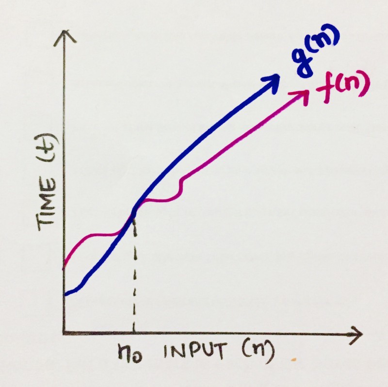
Let’s consider an algorithm which can be described by a function f(n). So, to define the BigO of f(n), we need to find a function, let’s say, g(n), which bounds it. Meaning, after a certain value, n0, the value of g(n) would always exceed f(n).

We can write it as,
f(n) ≤ C g(n)
where n≥n0; C> 0; n0≥1

If above conditions are fulfilled, we can say that g(n) is the BigO of f(n), or
f(n) = O (g(n))

Can we apply the same to analyze an algorithm? This basically means that in worst case scenario of running an algorithm, the value should not pass beyond a certain point, which is g(n) in this case. Hence, g(n) is the BigO of f(n).

Let’s go through some commonly used bigO notations and their complexity and understand them a little better.

• O(1): Describes an algorithm that will always execute in the same time (or space) regardless of the size of the input data set.

function firstItem(arr){      return arr[0];}

The above function firstItem(), will always take the same time to execute, as it returns the first item from an array, irrespective of its size. The running time of this function is independent of input size, and so it has a constant complexity of O(1).

Relating it to the above explanation, even in the worst case scenario of this algorithm (assuming input to be extremely large), the running time would remain constant and not go beyond a certain value. So, its BigO complexity is constant, that is O(1).

• O(N): Describes an algorithm whose performance will grow linearly and in direct proportion to the size of the input data set. Take a look at the example below. We have a function called matchValue() which returns true whenever a matching case is found in the array. Here, since we have to iterate over the whole of the array, the running time is directly proportional to the size of the array.

function matchValue(arr, k){   for(var i = 0; i < arr.length; i++){     if(arr[i]==k){       return true;     }     else{       return false;     }   }   }

This also demonstrates how Big O favors the worst-case performance scenario. A matching case could be found during any iteration of the for loop and the function would return early. But Big O notation will always assume the upper limit (worst-case) where the algorithm will perform the maximum number of iterations.

• O(N²): This represents an algorithm whose performance is directly proportional to the square of the size of the input data set. This is common with algorithms that involve nested iterations over the data set. Deeper nested iterations will result in O(N³), O(N⁴), etc.

function containsDuplicates(arr){    for (var outer = 0; outer < arr.length; outer++){        for (var inner = 0; inner < arr.length; inner++){            if (outer == inner)                 continue;            if (arr[outer] == arr[inner])                return true;        }    }       return false;}

• O(2^N): Denotes an algorithm whose growth doubles with each addition to the input data set. The growth curve of an O(2^N) function is exponential — starting off very shallow, then rising meteorically. An example of an O(2^N) function is the recursive calculation of Fibonacci numbers:

function recursiveFibonacci(number){    if (number <= 1) return number;    return recursiveFibonacci(number - 2) + recursiveFibonacci(number - 1);}

Are you getting the hang of this? Perfect. If not, feel free to fire up your queries in the comments below. :)

Moving on, now that we have a better understanding of the BigO notation, let us get to the next type of asymptotic analysis which is, the Big Omega(Ω).

The Big Omega (Ω)?
The Big Omega(Ω) provides us with the best case scenario of running an algorithm. Meaning, it would give us the minimum amount of resources (time or space) an algorithm would take to run.

Let’s dive into the mathematics of it to analyze it graphically.

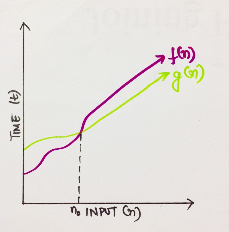
We have an algorithm which can be described by a function f(n). So, to define the BigΩ of f(n), we need to find a function, let’s say, g(n), which is tightest to the lower bound of f(n). Meaning, after a certain value, n0, the value of f(n) would always exceed g(n).

We can write it as,
f(n)≥ C g(n)
where n≥n0; C> 0; n0≥1

If above conditions are fulfilled, we can say that g(n) is the BigΩ of f(n), or
f(n) = Ω (g(n))

Can we infer that Ω(…) is complementary to O(…)? Moving on to the last section of this post…

The Big Theta (θ)?
The Big Theta(θ) is a sort of a combination of both BigO and BigΩ. It gives us the average case scenario of running an algorithm. Meaning, it would give us the mean of the best and worst case. Let’s analyse it mathematically.

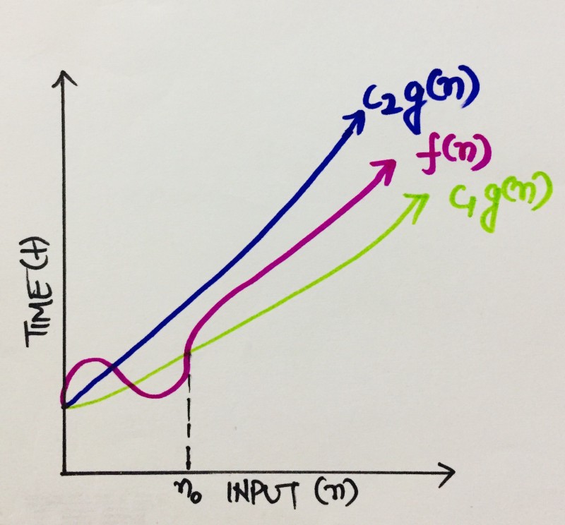
Considering an algorithm which can be described by a function f(n). The Bigθ of f(n) would be a function, let’s say, g(n), which bounds it the tightest by both lower and upper bound, such that,
C₁g(n) ≤ f(n)≤ C₂ g(n)
where C₁, C₂ >0, n≥ n0,
n0 ≥ 1

Meaning, after a certain value, n0, the value of C₁g(n) would always be less than f(n), and value of C₂ g(n) would always exceed f(n).

Now that we have a better understanding of the different types of asymptotic complexities, let’s have an example to get a clearer idea of how all this works practically.

Consider an array, of size, say, n, and we want to do a linear search to find an element x in it. Suppose the array looks something like this in the memory.

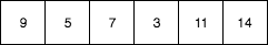
Going by the concept of linear search, if x=9, then that would be the best case scenario for the following case (as we don’t have to iterate over the whole array). And from what we have just learned, the complexity for this can be written as Ω(1). Makes sense?

Similarly, if x were equal to 14, that would be the worst case scenario, and the complexity would have been O(n).

What would be the average case complexity for this?
θ(n/2) => 1/2 θ(n) => θ(n) (As we ignore constants while calculating asymptotic complexities).

So, there you go folks. A fundamental insight into algorithmic complexities. Did it go well with you? Leave your advice, questions, suggestions in the comments below. Thanks for reading!❤️

References:-

• A nice write-up by Dionysis “dionyziz” Zindros: https://discrete.gr/complexity/
• A good series on algorithm & data structures: http://interactivepython.org/runestone/static/pythonds/AlgorithmAnalysis/WhatIsAlgorithmAnalysis.html