

How do you solve an ‘unsolvable’ problem?
The worlds of data science, mathematical finance, physics, engineering and bioinformatics (amongst many others) readily produce intractable problems. These are problems for which no computationally ‘easy’ solutions are available.
Luckily, there are methods that can approximate the solutions to these problems with a remarkably simple trick.
Monte Carlo methods are a class of methods that can be applied to computationally ‘difficult’ problems to arrive at near-enough accurate answers. The general premise is remarkably simple:
- Randomly sample input(s) to the problem
- For each sample, compute an output
- Aggregate the outputs to approximate the solution
As an analogy, imagine you’re an ant crawling over a large, tiled mosaic. From your vantage point, you have no easy way of working out what the mosaic depicts.
If you started walking around the mosaic and sampling the tiles you visit at random intervals, you’d build up an approximate idea of what the mosaic shows. The more samples you take, the better your approximation will be.
If you could cover every single tile, you’d eventually have a perfect representation of the mosaic. However, this wouldn’t be necessary — after a certain amount of sampling, you’d have a pretty good estimate.
This is exactly how Monte Carlo methods approximate solutions to otherwise ‘unsolvable’ problems.
The name refers to a famous casino in Monaco. It was coined in 1949 by one of the method’s pioneers, Stanislaw Ulam. Ulam’s uncle was reportedly a gambling man, and the connection between the element of ‘chance’ in gambling and in Monte Carlo methods must have been particularly apparent to Stanislaw.
The best way to understand a technical concept is to dive right in and see how it works. The rest of this article will show how Monte Carlo methods can solve three interesting problems. The examples will be presented in the Julia programming language.
Introducing Julia
There are a number of languages you might consider learning if you are interested in specialising in data science. One which has emerged as an increasingly serious option in recent years is a language called Julia.
Julia is a numerical programming language that has seen adoption within a range of quantitative disciplines. It is free to download. There’s also a really neat browser-based interface called JuliaBox, which is powered by Jupyter Notebook.
One of the cool features of Julia we’ll be making use of today is how easily it facilitates parallel computing. This allows you to carry out computations on multiple processes, giving a serious performance boost when done at scale.
Going parallel
To launch Julia on multiple processes, go to the terminal (or open a new terminal session in JuliaBox) and run the following command:
$ julia -p 4This initiates a Julia session on four CPUs. To define a function in Julia, the following syntax is used:
function square(x) return x^2 endThat’s right — instead of indentations or curly braces, Julia uses a start-end approach. For-loops are similar:
for i = 1:10 print(i) endYou can of course add whitespace and indentation to aid readability.
Julia’s parallel programming capabilities rely primarily upon two concepts: remote references and remote calls.
- Remote references are objects that essentially act as named placeholders for objects defined on other processes.
- Remote calls allow processes to call functions on arguments stored on other processes.
It is important to define functions across all processes. Check out the code below:
@everywhere function hello(x)
    return "Hello " * x
    end

result = @spawn hello("World!")
print(result)
fetched = fetch(result)
print(fetched)
The @everywhere macro ensures the hello() function is defined across all processes. The @spawn macro is used to wrap a closure around the expression hello("World!"), which is then evaluated remotely on an automatically chosen process.
The result of that expression is instantly returned as a Future remote reference. If you try printing result, you’ll be disappointed. The output of hello("World!") has been evaluated on a different process, and isn’t available here. To make it available, use the fetch() method.
If spawning and fetching seem like too much to bother with, then you’re in luck. Julia also has a @parallel macro that will take on some of the heavy lifting required for running tasks in parallel.
@parallel works either standalone, or with a ‘reducer’ function to collect the results across all processes and reduce them to a final output. Take a look at the code below:
@parallel (+) for i = 1:1000000000
    return i
    end
The for-loop simply returns the value of i at each step. The @parallel macro uses the addition operator as a reducer. It takes each value of i and adds it on to the previous values.
The result is the sum of the first billion integers.
With that whistle-stop tour of Julia’s parallel programming capabilities in mind, let’s move on to seeing how we can use Monte Carlo methods to solve some interesting example problems.
Playing the lottery
As a first example, let’s imagine playing a lottery game. The idea is simple — pick six unique numbers between 1 and 50. Each ticket costs, say, £2.
- If you match all six numbers to those drawn, you win a large prize (£1,000,000)
- If you match five numbers, you win a medium prize (£100,000)
- If you match four numbers, you win a small prize (£100)
- If you match three numbers, you win a very small prize (£10)
What would you expect to win if you played this lottery every day for twenty years?
You could work this out with pen and paper, by using a little probability theory. But that’d be time consuming! Instead, why not use a Monte Carlo method?
The approach is almost suspiciously simple — simulate the game over and over many times, and average the outcome.
Start Julia:
$ julia -p 4Now, import the StatsBase package. Use the @everywhere macro to make it available… well, everywhere.
using StatsBase@everywhere using StatsBaseNext, define a function that will simulate a single lottery game. The arguments allow you to change the rules of the game, to explore different scenarios.
@everywhere function lottery(n, outOf, price)
    ticket = sample(1:outOf, n, replace = false)
    draw = sample(1:outOf, n, replace = false)
    matches = sum(indexin(ticket,draw) .!= 0 )
    if matches == 6
        return 1000000 - price
    elseif matches == 5
        return 100000 - price
    elseif matches == 4
        return 100 - price
    elseif matches == 3
        return 10 - price
    else
        return 0 - price
    end
    end
The number of matching numbers is calculated using Julia’s indexin() function. This takes an array, and for each element, returns the index of its position in another array (or zero if the element is not found). Unlike many modern languages, Julia indexes from one, not zero.
The .!= 0 syntax checks which of these indices are not equal to zero, and returns either true or false for each. Finally, the number of true’s are summed up, giving the total matching numbers.
Now let’s simulate playing the lottery every day for twenty years… ten thousand times in parallel.
winnings = @parallel (+) for i = 1:(365*20*10000)
    lottery(6,50,2)
    end

print(winnings/10000)
Not a great return, huh?
You could extend the code to allow for more advanced rules and scenarios, and see the effect this has on the outcome.
Monte Carlo simulations allow for the modelling of considerably more complex situations than this lottery example. However, the approach is much the same as presented here.
Let’s see what else Monte Carlo methods allow us to do…
The value of pi
Pi (or π) is a mathematical constant. It is perhaps most famous for its appearance in the formula for the area of a circle:
A = πr²
π is an example of an irrational number. Its exact value is impossible to represent as any fraction of two integers. In fact, π is also an example of a transcendental number — there aren’t even any polynomial equations to which it is a solution.
You might think this makes obtaining an accurate value for π less-than-straightforward. Or does it?
Actually, you can find a pretty good estimate of π using a Monte Carlo-inspired method. A visual analogy might go as follows:
- Draw a 2m×2m square on a wall. Inside, draw a circle of radius 1m.
- Now, take a few steps back and hurl paint randomly at the wall. Count each time the paint lands in the circle.
- After a hundred throws, work out what fraction of throws landed in the circle. Multiply this by the area of the square. There is your estimate for π.
The reason this works is very intuitive.When sampling random points from a square containing a circle, the probability of selecting points from within the circle is proportional to the circle’s area.
With enough random samples, we can find a reliable estimate for this proportion, p.
Now, we know the area of the square is 2×2 = 4m², and we know the area of the circle is π×r². Since the radius r equals 1, the area of the circle is just π.
As we know the area of the square and have an estimate for the proportion p of its area covered by the circle, we can estimate π. Simply multiply p×4.
The more random samples we throw, the better the estimate p will be. However, the gain in accuracy diminishes as we take more and more samples.
Here’s the Julia code for simulating this example. I ran this in the JuliaBox terminal, using the following command to launch Julia on four CPUs:
$ julia -p 4First, define a sampling method.
@everywhere function throwPaint(N)
    hits = 0
    for i = 1:N
        x = rand() ; y = rand()
        if x^2 + y^2 < 1
            hits += 1
        end
    end
    return float(hits / N * 4)
end
This runs a loop, randomly sampling x and y coordinates between 0 and 1. The if-statement uses the circle equation to check if the points lie within an imaginary circle, counting the number of hits. The function returns the proportion of hits, multiplied by four.
Running this function in parallel will allow for an extremely high number of samples to be drawn, giving much greater precision.
Pi = @parallel (+) for i = 1:nworkers()
    throwPaint(100000000) / nworkers()
    end

print(Pi)
The nworkers() method returns the number of CPUs in use (in this case, four). This means each process runs the throwPaint() method, a hundred million times. Overall, this gives us a huge number of samples, and makes for a very precise estimate of the value of π.
The bigger picture: Integration
The estimating π example above is a specific example of a more general use case for Monte Carlo approximation — solving integration problems.
Integration is a calculus technique that finds an area defined by a mathematical function. For example, a simple curve might be defined by the function:
f(x) → x²
And the corresponding graph would be:
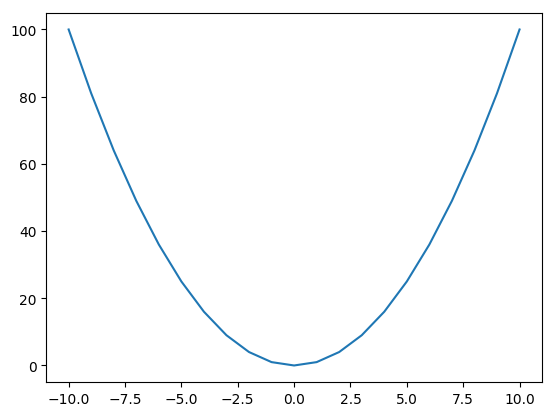
The area underneath the curve is found by integrating f(x).
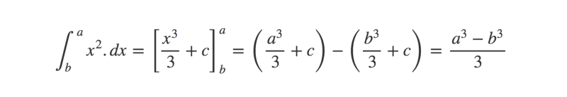
For simpler functions, integration is pretty easy to solve with a little practice. However, for more complicated functions, we need to turn to estimation methods.
In low dimensions, the area under a curve can be approximated by relatively simple algorithms, such as the trapezium method.
However, because of the curse of dimensionality, this becomes computationally unfeasible in higher dimensions. Monte Carlo-based methods can be used to estimate the area instead.
This can be visualized in exactly the same way as the π example above, except the curve need not be defined as a circle. Instead, imagine throwing paint at a unit square containing any arbitrary shape. For example:
In higher dimensions, the premise remains the same. The problem is still solved by randomly sampling input values, evaluating them, and aggregating to approximate the solution. Instead of sampling from a circle within a square, imagine sampling a sphere within a cube.
As a final example, let’s take on a difficult math puzzle.
A difficult math puzzle
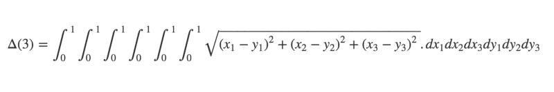
Pick two points at random within a unit cube. On average, what is the distance between them?
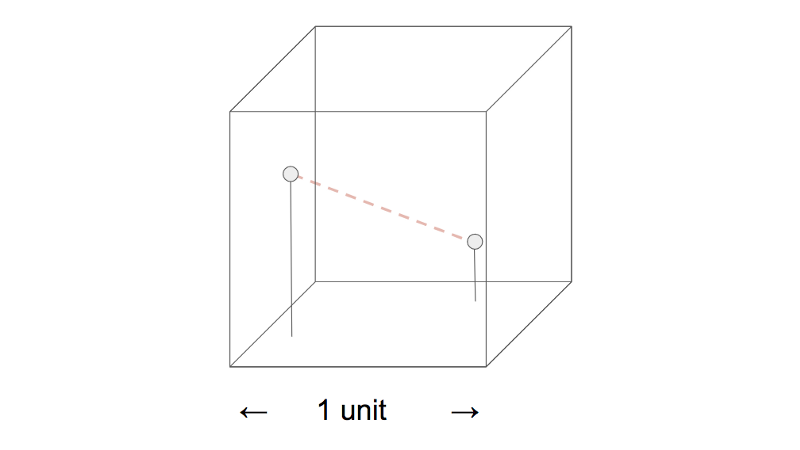
I’ll give you a warning now — the math solution isn’t exactly trivial.
However, it is possible to obtain an accurate estimate using — you guessed it — a Monte Carlo method.
$ julia -p 4First, define a sampling method.
@everywhere function samplePoints(dimensions)
    pt1 = []
    pt2 = []
    for i = 1:dimensions
        pt1 = push!(pt1, rand())
        pt2 = push!(pt2, rand())
    end
    return [pt1, pt2]
    end
Now define a function that calculates the distance between the points.
@everywhere function distance(points)
    pt1 = points[1]
    pt2 = points[2]
    arr = []
    for i = 1:length(pt1)
        d = (pt2[i] - pt1[i]) ^ 2
        arr = push!(arr, d)
    end
    dist = sqrt(sum(arr))
    return dist
    end
Finally, run these two functions together in parallel. Instead of reducing to a single output, this time we’ll write each result to a SharedArray object. SharedArray objects allow different processes to access data stored in the same array object.
results = SharedArray{Float64}(1000000)
@parallel for i = 1:1000000
    results[i] = distance(samplePoints(3))
    end

sum(results) / length(results)
You should get an answer very close to 0.6617 — and this is of course the correct answer! By changing the argument passed to samplePoints(), you can solve the generalised problem in however many dimensions you like.
What next?
Hopefully you’ve found this intro to Monte Carlo methods useful!
When implemented correctly, they provide an invaluable tool for data scientists, engineers, financial mathematicians and researchers… and anyone else whose work involves understanding complex systems.
If you’re interested in learning more about their applications, there’s a ton of resources online. However, the best way to learn is practice! Once you’re comfortable with the basic premise, why not have a go simulating your own Monte Carlo examples?
Any feedback or comments, please leave below!