by James Le

Spotify’s “This Is” playlists: the ultimate song analysis for 50 mainstream artists

Each artist has their own unique musical styles. From Ed Sheeran who devotes his life to the acoustic guitar, to Drake who masters the art of rapping. From Adele who can belt some crazy high notes on her pop ballads, to Kygo who creates EDM magic on his DJ set. Music is about creativity, originality, inspiration, and feelings, and it is the perfect gateway to connect people across differences.

Spotify is the largest music streaming service available. With more than 35 million songs and 170 million monthly active users, it is the ideal platform for musicians to reach their audience. On the app, music can be browsed or searched via various parameters — such as artists, album, genre, playlist, or record label. Users can create, edit, and share playlists, share tracks on social media, and make playlists with other users.

Additionally, Spotify launched a variety of interesting playlists tailor-made for its users, of which I most admire these three:

• Discover Weekly: a weekly generated playlist (updated on Mondays) that brings users two hours of custom-made music recommendations, mixing a user’s personal taste with songs enjoyed by similar listeners.
• Release Radar: a personalized playlist that allows users to stay up-to-date on new music released by artists they listen to the most.
• Daily Mix: a series of playlists that have “near endless playback” and mixes the user’s favorite tracks with new, recommended songs.

I recently discovered the ‘This Is” playlist series. One of Spotify’s best original features, “This Is” delivers on a major promise of the streaming revolution — the canonization and preservation of great artists’ repertoires for future generations to discover and appreciate.

Each one is dedicated to a different legendary artist, chronicling the high points of iconic discographies. “This is: Kanye West”. “This is: Maroon 5”. “This is: Elton John”. Spotify has provided a shortcut, giving us curated lists of the greatest songs from the greatest artists.

What we’ll cover here

The purpose of this project is to analyze the music that different artists on Spotify produce. The focus will be placed on disentangling the musical taste of 50 different artists from a wide range of genres. Throughout the process, I also identify different clusters of artists that share a similar musical style.

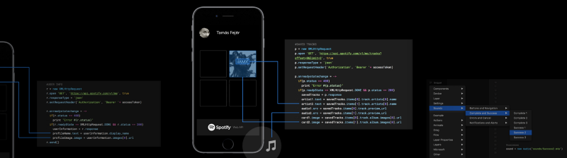
For the study, I will access the Spotify Web API, which provides data from the Spotify music catalog. This can be accessed via standard HTTPS requests to an API endpoint.

The Spotify API provides, among other things, track information for each song, including audio statistics such as danceability, instrumentalness, or tempo. Each feature measures an aspect of a song. Detailed information on how each feature is calculated can be found in the Spotify API Website. The code snippets in this article might be a bit tricky to understand, especially for data beginners, so bear with me.

Here’s a quick summary of my approach:

• Get the data from Spotify API.
• Process the data to extract audio features for each artist.
• Visualize the data using D3.js.
• Apply k-means clustering to separate the artists into different groups.
• Analyze each feature for all the artists.

Let’s now retrieve the audio feature information from “This Is” Playlists of 50 different artists on Spotify.

Getting data

The first step was registering my application in the API Website and getting the keys (Client ID and Client Secret) for future requests.

The Spotify Web API has different URIs (Uniform Resource Identifiers) to access playlists, artists, or tracks information. Consequently, the process of getting data must be divided into two key steps:

• get the “This Is” Playlist Series for multiple musicians.
• get the audio features for each artist’s Playlist tracks.

Web API credentials

First, I created two variables for the Client ID and the Client Secret credentials.

spotifyKey <- "YOUR CLIEND ID"spotifySecret <- "YOUR CLIENT SECRET"

After that, I requested an access token in order to authorize my app to retrieve and manage Spotify data.

library(Rspotify)library(httr)library(jsonlite)spotifyEndpoint <- oauth_endpoint(NULL, "https://accounts.spotify.com/authorize","https://accounts.spotify.com/api/token")

spotifyToken <- spotifyOAuth("Spotify Analysis", spotifyKey, spotifySecret)

“This Is” Playlist Series

The first step was to pull the artists’ “This Is” series is to get the URIs for each one. Here are the 50 musicians I have chosen, using their popularity, modernity, and diversity as the main criteria:

• Pop: Taylor Swift, Ariana Grande, Shawn Mendes, Maroon 5, Adele, Justin Bieber, Ed Sheeran, Justin Timberlake, Charlie Puth, John Mayer, Lorde, Fifth Harmony, Lana Del Rey, James Arthur, Zara Larsson, Pentatonix.
• Hip-Hop / Rap: Kendrick Lamar, Post Malone, Drake, Kanye West, Eminem, Future, 50 Cent, Lil Wayne, Wiz Khalifa, Snoop Dogg, Macklemore, Jay-Z.
• R & B: Bruno Mars, Beyonce, Enrique Iglesias, Stevie Wonder, John Legend, Alicia Keys, Usher, Rihanna.
• EDM / House: Kygo, The Chainsmokers, Avicii, Marshmello, Calvin Harris, Martin Garrix.
• Rock: Coldplay, Elton John, One Republic, The Script, Jason Mraz.
• Jazz: Frank Sinatra, Michael Buble, Norah Jones.

I basically went to each musician’s individual playlist, copied the URIs, stored each URI in a .csv file, and imported the .csv files into R.

library(readr)

playlistURI <- read.csv("this-is-playlist-URI.csv", header = T, sep = ";")

With each Playlist URI, I applied the getPlaylistSongs from the “RSpotify” package, and stored the Playlist information in an empty data.frame.

# Empty dataframePlaylistSongs <- data.frame(PlaylistID = character(),                            Musician = character(),                            tracks = character(),                            id = character(),                            popularity = integer(),                            artist = character(),                            artistId = character(),                            album = character(),                            albumId = character(),                            stringsAsFactors=FALSE)

# Getting each playlistfor (i in 1:nrow(playlistURI)) {  i <- cbind(PlaylistID = as.factor(playlistURI[i,2]),             Musician = as.factor(playlistURI[i,1]),             getPlaylistSongs("spotify",                              playlistid = as.factor(playlistURI[i,2]),                              token=spotifyToken))  PlaylistSongs <- rbind(PlaylistSongs, i)} 

Audio features

First, I wrote a formula (getFeatures) that extracts the audio features for any specific ID stored as a vector.

getFeatures <- function (vector_id, token) {  link <- httr::GET(paste0("https://api.spotify.com/v1/audio-features/?ids=",   vector_id), httr::config(token = token))  list <- httr::content(link)  return(list)}

Next, I included getFeatures in another formula (get_features). The latter formula extracts the audio features for the track ID’s vector, and returns them in a data.frame.

get_features <- function (x) {  getFeatures2 <- getFeatures(vector_id = x, token = spotifyToken)  features_output <- do.call(rbind, lapply(getFeatures2$audio_features, data.frame, stringsAsFactors=FALSE))}

Using the formula created above, I was able to extract the audio features for each track. In order to do so, I needed a vector containing each track ID. The rate limit for the Spotify API is 100 tracks, so I decided to create a vector with track IDs for each musician.

Next, I applied the get_features formula to each vector, obtaining the audio features for each musician.

After that, I merged each musician’s audio features data.frame into a new one, all_features. It contains the audio features for all the tracks in every musician’s “This Is” Playlist.

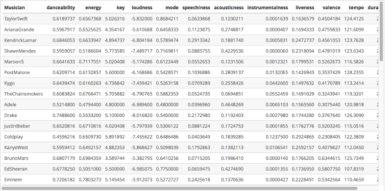
library(gdata)

all_features <- combine(TaylorSwift,ArianaGrande,KendrickLamar,ShawnMendes,Maroon5,PostMalone,Kygo,TheChainsmokers,Adele,Drake,JustinBieber,Coldplay,KanyeWest,BrunoMars,EdSheeran,Eminem,Beyonce,Avicii,Marshmello,CalvinHarris,JustinTimberlake,FrankSinatra,CharliePuth,MichaelBuble,MartinGarrix,EnriqueIglesias,JohnMayer,Future,EltonJohn,FiftyCent,Lorde,LilWayne,WizKhalifa,FifthHarmony,LanaDelRay,NorahJones,JamesArthur,OneRepublic,TheScript,StevieWonder,JasonMraz,JohnLegend,Pentatonix,AliciaKeys,Usher,SnoopDogg,Macklemore,ZaraLarsson,JayZ,Rihanna)

Finally, I computed the mean of each musician’s audio features using the aggregate function. The resulting data.frame contains the audio features for each musician, expressed as the mean of the tracks in their respective playlists.

mean_features <- aggregate(all_features[, c(1:11,17)], list(all_features$source), mean)

names(mean_features) <- c("Musician", "danceability", "energy", "key", "loudness", "mode", "speechiness", "acousticness", "instrumentalness", "liveness", "valence", "tempo", "duration_ms")

The image below shows a subset of the mean_features data.frame, for your reference.

Audio features description

The description of each feature from the Spotify Web API Guidance can be found below:

• Danceability: describes the suitability of a track for dancing. This is based on a combination of musical elements including tempo, rhythm stability, beat strength, and overall regularity. A value of 0.0 is least danceable and 1.0 is most danceable.
• Energy: a measure from 0.0 to 1.0, and represents a perceptual measure of intensity and activity. Typically, energetic tracks feel fast, loud, and noisy. For example, death metal has high energy, while a Bach prelude scores low on the scale. Perceptual features contributing to this attribute include dynamic range, perceived loudness, timbre, onset rate, and general entropy.
• Key: the key the track is in. Integers map to pitches using standard Pitch Class notation. E.g. 0 = C, 1 = C♯/D♭, 2 = D, and so on.
• Loudness: the overall loudness of a track in decibels (dB). Loudness values are averaged across the entire track and are useful for comparing the relative loudness of tracks. Loudness is the quality of a sound that is the primary psychological correlate of physical strength (amplitude). Values typical range between -60 and 0 db.
• Mode: indicates the modality (major or minor) of a track, the type of scale from which its melodic content is derived. Major is represented by 1 and minor is 0.
• Speechiness: Speechiness detects the presence of spoken words in a track. The more exclusively speech-like the recording (e.g. talk show, audio book, poetry), the closer to 1.0 the attribute value. Values above 0.66 describe tracks that are probably made entirely of spoken words. Values between 0.33 and 0.66 describe tracks that may contain both music and speech, either in sections or layered, including such cases as rap music. Values below 0.33 most likely represent instrumental music and other non-speech-like tracks.
• Acousticness: a confidence measure from 0.0 to 1.0 of whether the track is acoustic. 1.0 represents high confidence that the track is acoustic.
• Instrumentalness: predicts whether a track contains no vocals. “Ooh” and “aah” sounds are treated as instrumental in this context. Rap or spoken word tracks are clearly “vocal”. The closer the instrumentalness value is to 1.0, the greater likelihood the track contains no vocal content. Values above 0.5 are intended to represent instrumental tracks, but confidence is higher as the value approaches 1.0.
• Liveness: detects the presence of an audience in the recording. Higher liveness values represent an increased probability that the track was performed live. A value above 0.8 provides strong likelihood that the track is live.
• Valence: a measure from 0.0 to 1.0 describing the musical positiveness conveyed by a track. Tracks with high valence sound more positive (for example happy, cheerful, euphoric), while tracks with low valence sound more negative (for example sad, depressed, angry).
• Tempo: the overall estimated tempo of a track in beats per minute (BPM). In musical terminology, tempo is the speed or pace of a given piece, and derives directly from the average beat duration.
• Duration_ms: the duration of the track in milliseconds.

Data Visualization

Radar charts

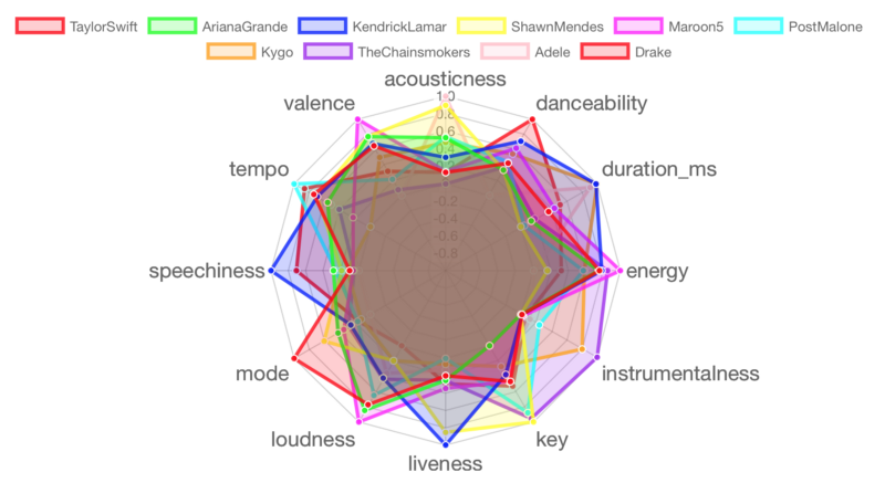
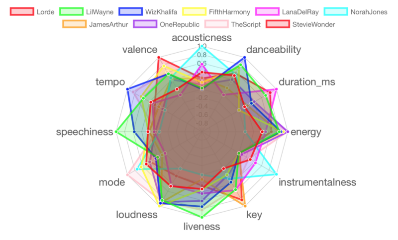
A radar chart is useful to compare the musical vibes of these musicians in a more visual way. The first visualization is an R implementation of the radar chart from the chart.js JavaScript library, and evaluates the audio features for ten selected musicians.

In order to plot, I normalized the key, loudness, tempo, and duration_ms values to be from 0 to 1. This helps to make the chart more clear and readable.

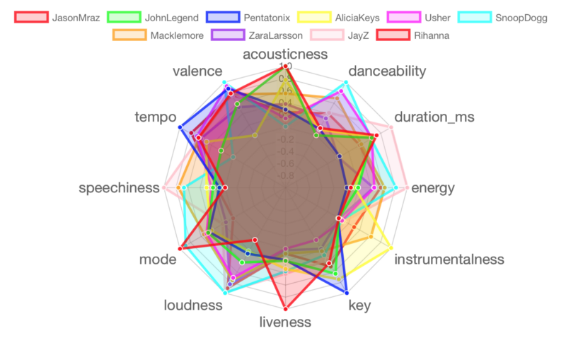
mean_features_norm <- cbind(mean_features[1], apply(mean_features[-1],2, function(x){(x-min(x))/diff(range(x))}))

Okay, let’s plot these interactive radar charts in batches of ten musicians. Each chart displays data set labels when you hover over each radial line, showing the value for the selected feature. The code below details the process of making the radar chart for the first batch of ten musicians. The code for the other four batches has been omitted, but the radar charts are displayed.

Batch 1: Taylor Swift, Ariana Grande, Kendrick Lamar, Shawn Mendes, Maroon 5, Post Malone, Kygo, The Chainsmokers, Adele, Drake

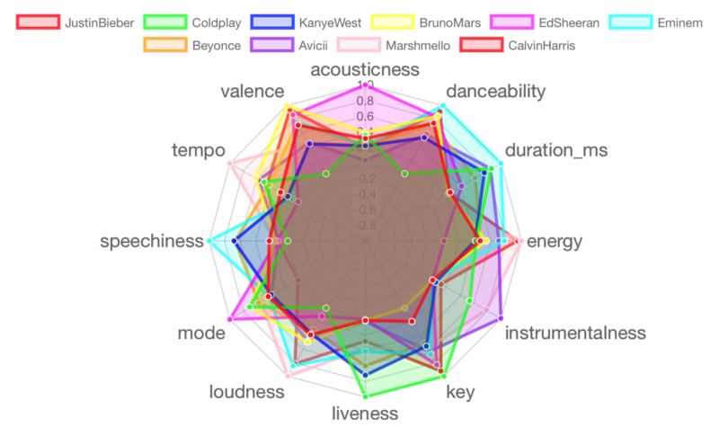
Batch 2: Justin Bieber, Coldplay, Kanye West, Bruno Mars, Ed Sheeran, Eminem, Beyonce, Avicii, Marshmello, Calvin Harris

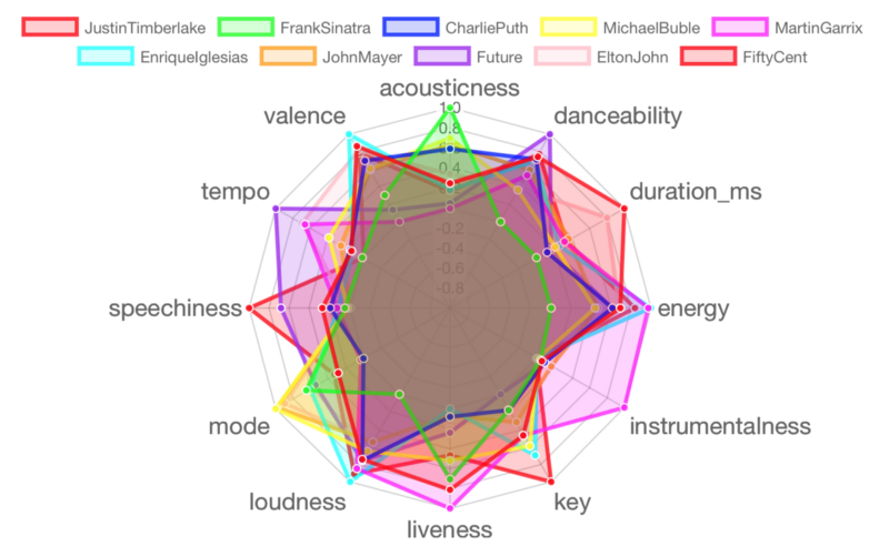
Batch 3: Justin Timberlake, Frank Sinatra, Charlie Puth, Michael Buble, Martin Garrix, Enrique Iglesias, John Mayer, Future, Elton John, 50 Cent

Batch 4: Lorde, Lil Wayne, Wiz Khalifa, Fifth Harmony, Lana Del Rey, Norah Jones, James Arthur, One Republic, The Script, Stevie Wonder

Batch 5: Jason Mraz, John Legend, Pentatonix, Alicia Keys, Usher, Snoop Dogg, Macklemore, Zara Larsson, Jay-Z, Rihanna

Cluster Analysis

Another way to find out the differences between these musicians in their musical repertoire is by grouping them in clusters. The general idea of a clustering algorithm is to divide a given dataset into multiple groups on the basis of similarity in the data.

In this case, musicians will be grouped in different clusters according to their music preferences. Rather than defining groups before looking at the data, clustering allows me to find and analyze the musician groupings that have formed organically.

Prior to clustering data, it is important to rescale the numeric variables of the dataset. Since I have mixed numerical data, where each audio feature is different from another and has different measurements, running the scale function (aka z-standardizing them) is a good practice to give equal weight to them. After that, I kept the musicians as the row names to be able to show them as labels in the plot.

scaled.features <- scale(mean_features[-1])rownames(scaled.features) <- mean_features$Musician

I applied the K-Means Clustering method, which is one of the most popular techniques of unsupervised statistical learning methods. It is used for unlabeled data. The algorithm finds groups in the data, with the number of groups represented by the variable K. The algorithm works iteratively to assign each data point to one of K groups based on the variables that are provided. Data points are clustered based on similarity.

In this instance, I chose K = 6 — the clusters can be formed based on the six different genres I used when choosing the artists (Pop, Hip-Hop, R&B, EDM, Rock, and Jazz).

After I applied the K-Means algorithm for each musician, I can plot a two-dimensional view of the data. In the first plot, the x-axis and y-axis correspond to the first and second principal components respectively. The eigenvectors (represented by red arrows) indicate the directional influence each variable has on the principal components.

Let’s have a look at the clusters that result from applying the K-Means algorithm to my dataset.

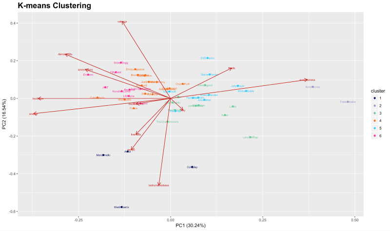
As you can see in the graph above, the x-axis is PC1 (30.24%) and the y-axis is PC2 (16.54%). These are the first two principal components. The PCA graph shows that PC1 separates artists by loudness/energy vs acoustic/mellowness, while PC2 appears to separate artists on a scale of valence vs key, tempo and instrumentalness.

Because my data is multivariate, it is tedious to inspect all the many bivariate scatterplots. Instead, a single “summarizing” scatterplot is more convenient. The scatterplot of the first two principal components which were derived from the data has been shown in the graph. The percentage, likewise, is the variance explained by each component of the overall variability: the 1st component captured 30.24% and the 2nd component captured 16.54% of the information about the multivariate data.

If you’re interested to learn more about the math behind this algorithm, I recommend that you brush up on Principal Component Analysis.

Let’s see which artists belong to which clusters:

k_means$cluster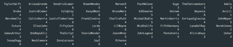

I have also plotted another radar chart containing the features for each cluster. It is useful to compare the attributes of the songs that each cluster creates.

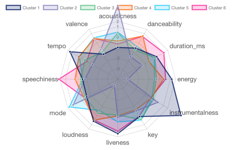
Cluster 1 contains four artists: Coldplay, Avicii, Marshmello, and Martin Garrix. Their music is mostly performed live and instrumental, usually loud and full of energy with high tempo. This is not too surprising, as three of the four artists perform EDM / House music, and Coldplay is known for their live concerts.

Cluster 2 contains 2 artists: Frank Sinatra and Norah Jones (any jazz fans out there?). Their music scores high on acousticness and the Major scale mode. However, they score low in all the remaining attributes. Typical Jazz tunes.

Cluster 3 contains ten artists: Post Malone, Kygo, The Chainsmokers, Adele, Lorde, Lana Del Rey, James Arthur, One Republic, John Legend, and Alicia Keys. This cluster scores average in mostly all the attributes. This suggests that this group of artists is well-balanced and versatile with style and creation, hence the diversity of genres presented in this cluster (EDM, Pop, R&B).

Cluster 4 contains 15 artists: Ariana Grande, Maroon 5, Drake, Justin Bieber, Bruno Mars, Calvin Harris, Charlie Puth, Enrique Iglesias, Future, Wiz Khalifa, Fifth Harmony, Usher, Macklemore, Zara Larsson, and Rihanna. Their music is danceable, loud, high-tempo, and energetic. This group has the presence of many young mainstream artists in the Pop and Hip-Hop genres.

Cluster 5 contains 10 artists: Taylor Swift, Shawn Mendes, Ed Sheeran, Michael Buble, John Mayer, Elton John, The Script, Stevie Wonder, Jason Mraz, and Pentatonix. This is my favorite group! Taylor Swift? Ed Sheeran? John Mayer? Jason Mraz? Elton John? I guess I listen to a lot of singer-songwriter artists. Their music is mostly in the Major scale, while achieving perfect balance (average score) in all other attributes.

Cluster 6 contains nine artists: Kendrick Lamar, Kanye West, Eminem, Beyonce, Justin Timberlake, 50 Cent, Lil Wayne, Snoop Dogg, and Jay-Z. You already see the trend here: seven of them are Rappers, and even Beyonce and JT regularly collaborate with rappers. Their songs have high number of spoken words and speech-like sections, are long in duration, and often performed live. Any better description of rap music?

Analysis by feature

The following charts show the values for each feature for every musician. The code below details the process for making the danceability diverging bar plot. The code for the other features has been omitted, but each feature’s plot is displayed subsequently.

Danceability

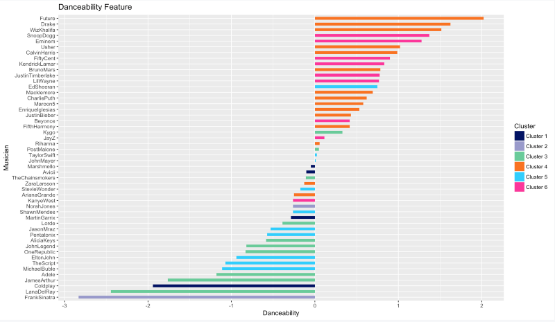
If you want to bust the moves and impress your crush, try listen to more of Future, Drake, Wiz Khalifa, Snoop Doog, and Eminem. On the other hand, don’t even attempt to dance to Frank Sinatra or Lana Del Rey’s tunes.

Energy

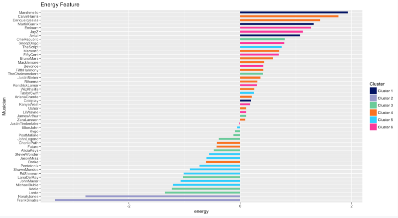
You’re a fairly energetic person if you listen to lots of Marhsmello, Calvin Harris, Enrique Iglesias, Martin Garrix, Eminem, Jay-Z. The opposite is true if you’re a fan of Frank Sinatra and Norah Jones.

Loudness

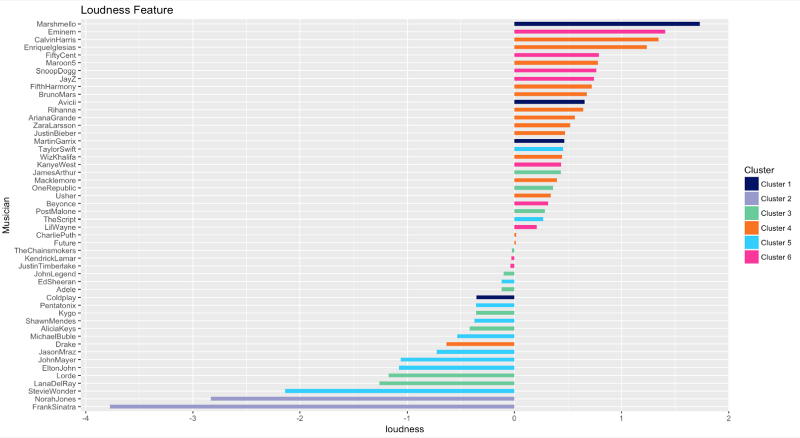
The Loudness ranking is almost the same as the Energy one.

Speechiness

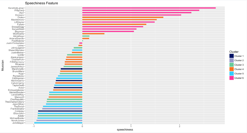
All the Rap fans out there: what’s your favorite songs from Kendrick Lamar? or 50 Cent? or Jay-Z? Hmm, I’m surprised Eminem does not rank higher, as I personally think that he’s the GOAT of all rappers.

Acousticness

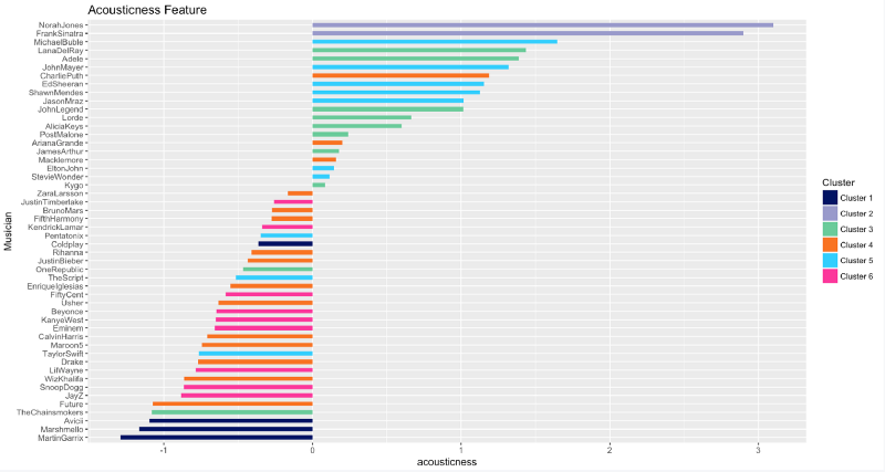
Acousticness is the exact opposite of Loudness and Energy. Mr. Sinatra and Mrs. Jones released some powerful acoustic tracks throughout their careers.

Instrumentalness

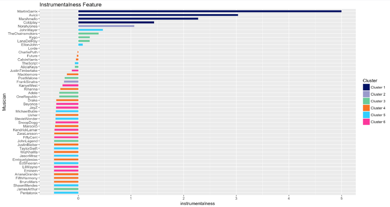
EDM for the win! Martin Garrix, Avicii, and Marshmello produce tracks that contain almost no vocals.

Liveness

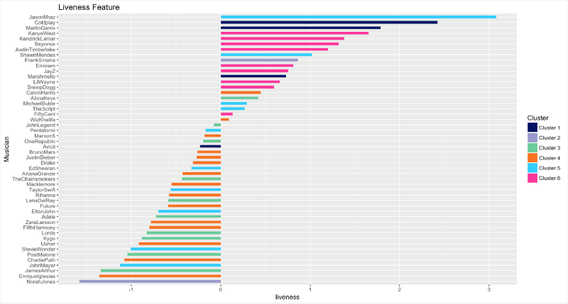
So who are the 5 artists who performed the most live audio recordings? Jason Mraz, Coldplay, Martin Garrix, Kanye West, and Kendrick Lamar, in that order.

Valence

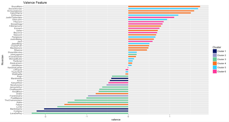
Valence is the feature that describes musical positiveness conveyed by a track. Music by Bruno Mars, Stevie Wonder, and Enrique Iglesias are very positive, while music by Lana Del Rey, Coldplay, and Martin Garrix sound quite negative.

Tempo

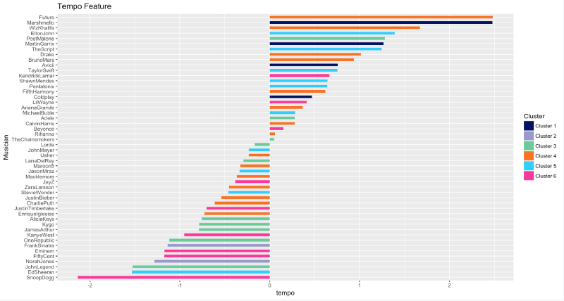
Future, Marshmello, and Wiz Khalifa are kings of speed. They produce tracks with the highest tempo in beats per minute. And Snoop Dogg, lol? He tends to take some time to utter his magic words.

Duration

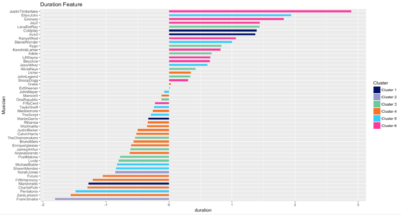
Last but not least, songs by Justin Timberlake, followed by Elton John and Eminem, are, sometimes excruciatingly, long. In contrast, Frank Sinatra, Zara Larsson, and Pentatonix favor shorter music.

Conclusion

Whoa, I had a lot of fun doing this analysis and visualization project on Spotify data. Who could have thought that James Arthur and Post Malone are in the same cluster? Or Kendrick Lamar is the speediest rapper in the game? Or that Marshmello would beat Martin Garrix in producing energetic tracks?

Anyway, you can view the complete R Markdown, separate R code for processing and visualizing data, and the original dataset in my GitHub repository here. From my own perspective, R is much better in data visualization than Python, with the likes of libraries such as ggplot and plot.ly. I highly encourage you to give R a try!

— —

If you enjoyed this piece, I’d love it if you hit the clap button ? so others might stumble upon it. You can find my own code on GitHub, and more of my writing and projects at https://jameskle.com/. You can also follow me on Twitter, email me directly or find me on LinkedIn. Sign up for my newsletter to receive my latest thoughts on data science, machine learning, and artificial intelligence right at your inbox!