by Nick Bourdakos
Tracking the Millennium Falcon with TensorFlow
At the time of writing this post, most of the big tech companies (such as IBM, Google, Microsoft, and Amazon) have easy-to-use visual recognition APIs. Some smaller companies also provide similar offerings, such as Clarifai. But none of them offer object detection.
Update: IBM and Microsoft now have customizable object detection APIs.
The following images were both tagged using the same Watson Visual Recognition default classifier. The first one, though, has been run through an object detection model first.
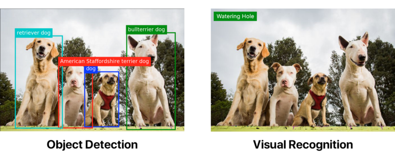
Object detection can be far superior to visual recognition on its own. But if you want object detection, you’re going to have to get your hands a little dirty.
Depending on your use case, you may not need a custom object detection model. TensorFlow’s object detection API provides a few models of varying speed and accuracy, that are based on the COCO dataset.
For your convenience, I have put together a complete list of objects that are detectable with the COCO models:
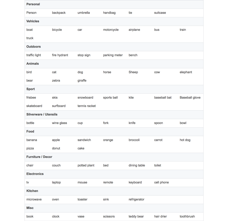
If you wanted to detect logos or something not on this list, you’d have to build your own custom object detector. I wanted to be able to detect the Millennium Falcon and some Tie Fighters. This is obviously an extremely important use case, because you never know…
Annotate your images
Training your own model is a lot of work. At this point, you may be thinking, “Whoa, whoa, whoa! I don’t want to do a lot of work!” If so, you can check out my other article about using the provided model. It’s a much smoother ride.
You need to collect a lot of images and annotate them all. Annotations include specifying the object coordinates and a corresponding label. For an image with two Tie Fighters, an annotation might look something like this:
<annotation> <folder>images</folder> <filename>image1.jpg</filename> <size> <width>1000</width> <height>563</height> </size> <segmented>0</segmented> <object> <name>Tie Fighter</name> <bndbox> <xmin>112</xmin> <ymin>281</ymin> <xmax>122</xmax> <ymax>291</ymax> </bndbox> </object> <object> <name>Tie Fighter</name> <bndbox> <xmin>87</xmin> <ymin>260</ymin> <xmax>95</xmax> <ymax>268</ymax> </bndbox> </object></annotation>For my Star Wars model, I collected 308 images including two or three objects in each. I’d recommend trying to find 200–300 examples of each object.
“Wow,” you might be thinking, “I have to go through hundreds of images and write a bunch of XML for each one?”
Of course not! There are plenty of annotation tools out there, such as labelImg and RectLabel. I used RectLabel, but it’s only for macOS. It’s still a lot of work, trust me. It took me about three or four hours of nonstop work to annotate my entire dataset.
Update: I ended up building my own tool to annotate images and video frames. It’s a free online tool called Cloud Annotations that you can check out here.
If you have the money, you can pay somebody else, like an intern, to do it. Or you can use something like Mechanical Turk. If you are a broke college student like me and/or find doing hours of monotonous work fun, you’re on your own.
We will need to do a little setup before we can run the script to prepare the data for TensorFlow.
Clone the repo
Start by cloning my repo here.
Update: This repo is a bit out of date, I recommend checking out this one for a much better time :)
Note: The following instructions are also out of date, I urge you to check out the new walkthrough.
The directory structure will need to look like this:
models|-- annotations| |-- label_map.pbtxt| |-- trainval.txt| `-- xmls| |-- 1.xml| |-- 2.xml| |-- 3.xml| `-- ...|-- images| |-- 1.jpg| |-- 2.jpg| |-- 3.jpg| `-- ...|-- object_detection| `-- ...`-- ...I’ve included my training data, so you should be able to run this out of the box. But if you want to create a model with your own data, you’ll need to add your training images to images, add your XML annotations to annotations/xmls, update trainval.txt, and label_map.pbtxt.
trainval.txt is a list of file names that allows us to find and correlate the JPG and XML files. The following trainval.txt list would let us to find abc.jpg, abc.xml, 123.jpg, 123.xml, xyz.jpg and xyz.xml:
abc123xyzNote: Make sure your JPG and XML file names match, minus the extension.
label_map.pbtxt is our list of objects that we are trying to detect. It should look something like this:
item { id: 1 name: 'Millennium Falcon'}item { id: 2 name: 'Tie Fighter'}Running the script
First, with Python and pip installed, install the scripts requirements:
pip install -r requirements.txtAdd models and models/slim to your PYTHONPATH:
export PYTHONPATH=$PYTHONPATH:`pwd`:`pwd`/slimImportant Note: This must be run every time you open the terminal, or added to your ~/.bashrc file.
Run the script:
python object_detection/create_tf_record.pyOnce the script finishes running, you will end up with a train.record and a val.record file. This is what we will use to train the model.
Downloading a base model
Training an object detector from scratch can take days, even when using multiple GPUs. To speed up training, we’ll take an object detector trained on a different dataset and reuse some of it’s parameters to initialize our new model.
You can download a model from this model zoo. Each model varies in accuracy and speed. I used faster_rcnn_resnet101_coco.
Extract and move all the model.ckpt files to our repo’s root directory.
You should see a file named faster_rcnn_resnet101.config. It’s set to work with the faster_rcnn_resnet101_coco model. If you used another model, you can find a corresponding config file here.
Ready to train
Run the following script, and it should start to train!
python object_detection/train.py \ --logtostderr \ --train_dir=train \ --pipeline_config_path=faster_rcnn_resnet101.configNote: Replace pipeline_config_path with the location of your config file.
global step 1:global step 2:global step 3:global step 4:...Yay! It’s working!
10 minutes later.
global step 41:global step 42:global step 43:global step 44:...Computer starts smoking.
global step 71:global step 72:global step 73:global step 74:...How long is this thing supposed to run?
The model that I used in the video ran for about 22,000 steps.
Wait, what?!
I use a specked-out MacBook Pro. If you’re running this on something similar, I’ll assume you’re getting about one step every 15 seconds or so. At that rate it will take about three to four days of nonstop running to get a decent model.
Well, this is dumb. I don’t have time for this ?
PowerAI to the rescue!
PowerAI
PowerAI lets us train our model on IBM Power Systems with P100 GPUs fast!
It only took about an hour to train for 10,000 steps. However, this was just with one GPU. The real power in PowerAI comes from the the ability to do distributed deep learning across hundreds of GPUs with up to 95% efficiency.
With the help of PowerAI, IBM just set a new image recognition record of 33.8% accuracy in 7 hours. It surpassed the previous industry record set by Microsoft — 29.9% accuracy in 10 days.
WAYYY fast!
Since I’m not training on millions of images, I definitely didn’t need those kind of resources. One GPU will do.
Creating a Nimbix account
Nimbix provides developers a trial account with ten hours of free processing time on the PowerAI platform. You can register here.
Note: This process is not automated, so it may take up to 24 hours to be reviewed and approved.
Once approved, you should receive an email with instructions on confirming and creating your account. It will ask you for a promotional code, but leave it blank.
You should now be able to log in here.
Deploy the PowerAI Notebooks application
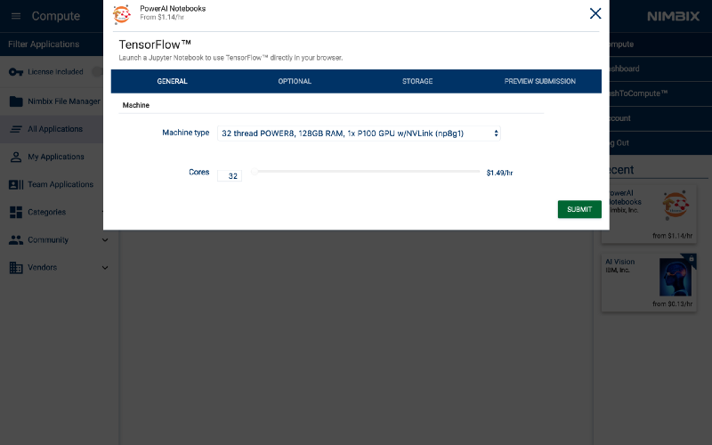
Start by searching for PowerAI Notebooks.
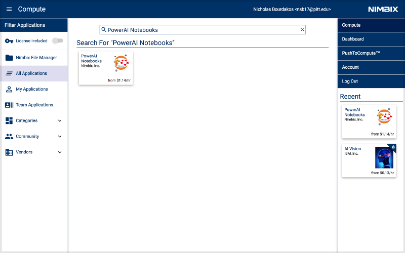
Click on it, and then choose TensorFlow.
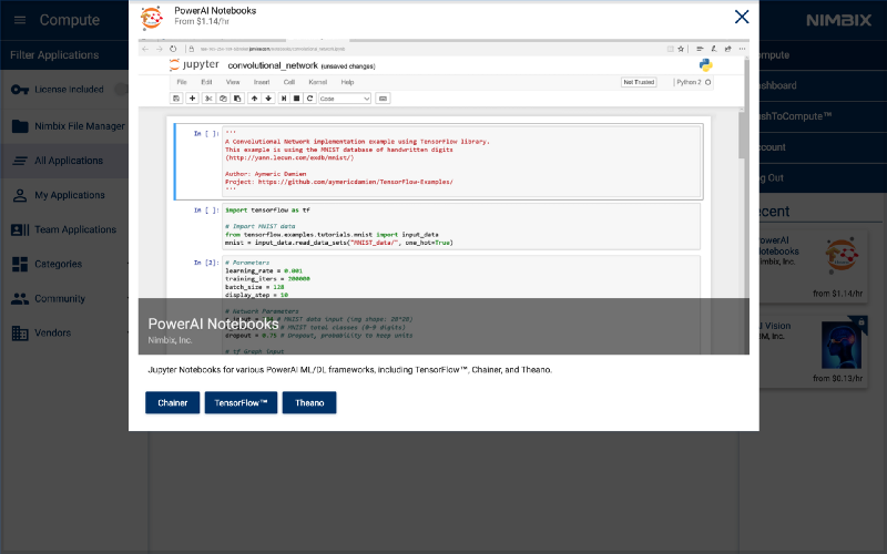
Choose the machine type of 32 thread POWER8, 128GB RAM, 1x P100 GPU w/NVLink (np8g1).
Once started, the following dashboard panel will be displayed. When the server Status turns to Processing, the server is ready to be accessed.
Get the password by clicking on (click to show).
Then, click Click here to connect to launch the Notebook.
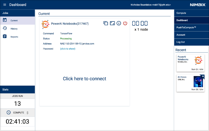
Log-in using the user name nimbix and the previously supplied password.

Start training
Get a new terminal window by clicking on the New pull-down and selecting Terminal.

You should be greeted with a familiar face:
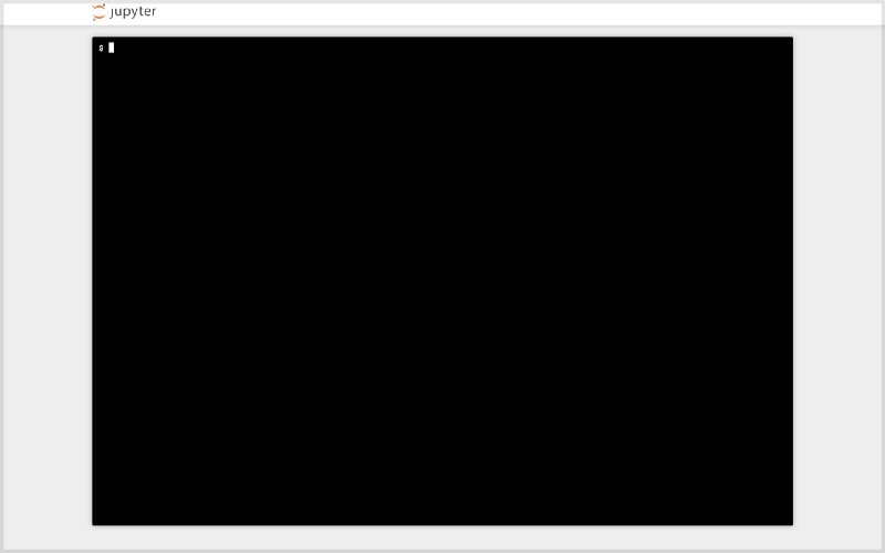
Note: Terminal may not work in Safari.
The steps for training are the same as they were when we ran this locally. If you’re using my training data then you can just clone my repo by running (if not, just clone your own repo):
git clone https://github.com/bourdakos1/Custom-Object-Detection.gitThen cd into the root directory:
cd Custom-Object-DetectionRun this snippet, which will download the pre-trained faster_rcnn_resnet101_coco model we downloaded earlier.
wget http://storage.googleapis.com/download.tensorflow.org/models/object_detection/faster_rcnn_resnet101_coco_11_06_2017.tar.gztar -xvf faster_rcnn_resnet101_coco_11_06_2017.tar.gzmv faster_rcnn_resnet101_coco_11_06_2017/model.ckpt.* .Then we need to update our PYTHONPATH again, because this in a new terminal:
export PYTHONPATH=$PYTHONPATH:`pwd`:`pwd`/slimThen we can finally run the training command again:
python object_detection/train.py \ --logtostderr \ --train_dir=train \ --pipeline_config_path=faster_rcnn_resnet101.configDownloading your model
When is my model ready? It depends on your training data. The more data, the more steps you’ll need. My model was pretty solid at nearly 4,500 steps. Then, at about 20,000 steps, it peaked. I even went on and trained it for 200,000 steps, but it didn’t get any better.
I recommend downloading your model every 5,000 steps or so and evaluating it to make sure you’re on the right path.
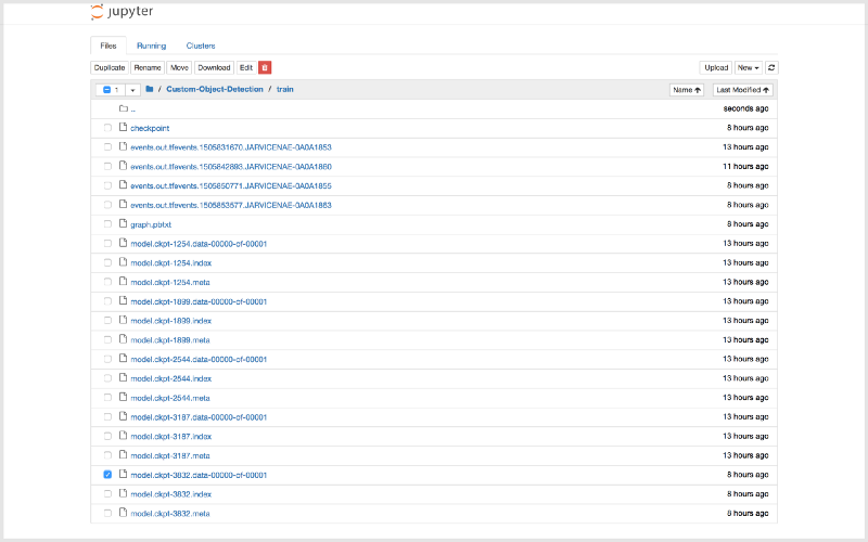
Click on the Jupyter logo in the top left corner. Then, navigate the file tree to Custom-Object-Detection/train.
Download all the model.ckpt files with the highest number.
model.ckpt-STEP_NUMBER.data-00000-of-00001model.ckpt-STEP_NUMBER.indexmodel.ckpt-STEP_NUMBER.meta
Note: You can only download one at a time.
Note: Be sure to click the red power button on your machine when finished. Otherwise, the clock will keep on ticking indefinitely.
Export the inference graph
To use the model in our code, we need to convert the checkpoint files (model.ckpt-STEP_NUMBER.*) into a frozen inference graph.
Move the checkpoint files you just downloaded into the root folder of the repo you’ve been using.
Then run this command:
python object_detection/export_inference_graph.py \ --input_type image_tensor \ --pipeline_config_path faster_rcnn_resnet101.config \ --trained_checkpoint_prefix model.ckpt-STEP_NUMBER \ --output_directory output_inference_graphRemember export PYTHONPATH=$PYTHONPATH:`pwd`:`pwd`/slim .
You should see a new output_inference_graph directory with a frozen_inference_graph.pb file. This is the file we need.
Test the model
Now, run the following command:
python object_detection/object_detection_runner.pyIt will run your object detection model found at output_inference_graph/frozen_inference_graph.pb on all the images in the test_images directory and output the results in the output/test_images directory.
The results
Here’s what we get when we run our model over all the frames in this clip from Star Wars: The Force Awakens.
Thanks for reading! If you have any questions, feel free to reach out at bourdakos1@gmail.com, connect with me on LinkedIn, or follow me on Medium and Twitter.
If you found this article helpful, it would mean a lot if you gave it some applause? and shared to help others find it! And feel free to leave a comment below.