by Nick Bourdakos
Understanding Capsule Networks — AI’s Alluring New Architecture

Convolutional neural networks have done an amazing job, but are rooted in problems. It’s time we started thinking about new solutions or improvements — and now, enter capsules.
Previously, I briefly discussed how capsule networks combat some of these traditional problems. For the past for few months, I’ve been submerging myself in all things capsules. I think it’s time we all try to get a deeper understanding of how capsules actually work.
In order to make it easier to follow along, I have built a visualization tool that allows you to see what is happening at each layer. This is paired with a simple implementation of the network. All of it can be found on GitHub here.
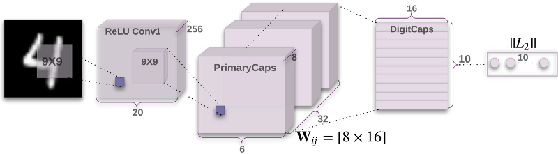
This is the CapsNet architecture. Don’t worry if you don’t understand what any of it means yet. I’ll be going through it layer by layer, with as much detail as I can possibly conjure up.
Part 0: The Input
The input into CapsNet is the actual image supplied to the neural net. In this example the input image is 28 pixels high and 28 pixels wide. But images are actually 3 dimensions, and the 3rd dimension contains the color channels.
The image in our example only has one color channel, because it’s black and white. Most images you are familiar with have 3 or 4 channels, for Red-Green-Blue and possibly an additional channel for Alpha, or transparency.
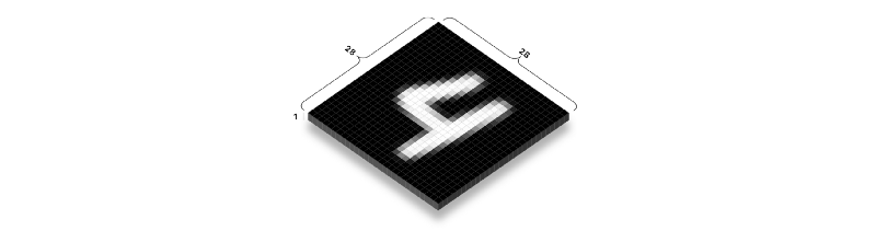
Each one of these pixels is represented as a value from 0 to 255 and stored in a 28x28x1 matrix [28, 28, 1]. The brighter the pixel, the larger the value.
Part 1a: Convolutions
The first part of CapsNet is a traditional convolutional layer. What is a convolutional layer, how does it work, and what is its purpose?
The goal is to extract some extremely basic features from the input image, like edges or curves.
How can we do this?
Let’s think about an edge:
If we look at a few points on the image, we can start to pick up a pattern. Focus on the colors to the left and right of the point we are looking at:
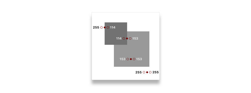
You might notice that they have a larger difference if the point is an edge:
255 - 114 = 141
114 - 153 = -39
153 - 153 = 0
255 - 255 = 0
What if we went through each pixel in the image and replaced its value with the value of the difference of the pixels to the left and right of it? In theory, the image should become all black except for the edges.
We could do this by looping through every pixel in the image:
for pixel in image {
  result[pixel] = image[pixel - 1] - image[pixel + 1]
}
But this isn’t very efficient. We can instead use something called a “convolution.” Technically speaking, it’s a “cross-correlation,” but everyone likes to call them convolutions.
A convolution is essentially doing the same thing as our loop, but it takes advantage of matrix math.
A convolution is done by lining up a small “window” in the corner of the image that only lets us see the pixels in that area. We then slide the window across all the pixels in the image, multiplying each pixel by a set of weights and then adding up all the values that are in that window.
This window is a matrix of weights, called a “kernel.”
We only care about 2 pixels, but when we wrap the window around them it will encapsulate the pixel between them.
Window:
┌─────────────────────────────────────┐
│ left_pixel middle_pixel right_pixel │
└─────────────────────────────────────┘
Can you think of a set of weights that we can multiply these pixels by so that their sum adds up to the value we are looking for?
Window:
┌─────────────────────────────────────┐
│ left_pixel middle_pixel right_pixel │
└─────────────────────────────────────┘
(w1 * 255) + (w2 * 255) + (w3 * 114) = 141
Spoilers below!
 │            │            │
 │            │            │
 │            │            │
 │            │            │
 │            │            │
\│/          \│/          \│/
 V            V            V
We can do something like this:
Window:
┌─────────────────────────────────────┐
│ left_pixel middle_pixel right_pixel │
└─────────────────────────────────────┘
(1 * 255) + (0 * 255) + (-1 * 114) = 141
With these weights, our kernel will look like this:
kernel = [1 0 -1]However, kernels are generally square — so we can pad it with more zeros to look like this:
kernel = [
  [0  0  0]
  [1  0 -1]
  [0  0  0]
]
Here’s a nice gif to see a convolution in action:
Note: The dimension of the output is reduced by the size of the kernel plus 1. For example:(7 — 3) + 1 = 5 (more on this in the next section)
Here’s what the original image looks like after doing a convolution with the kernel we crafted:
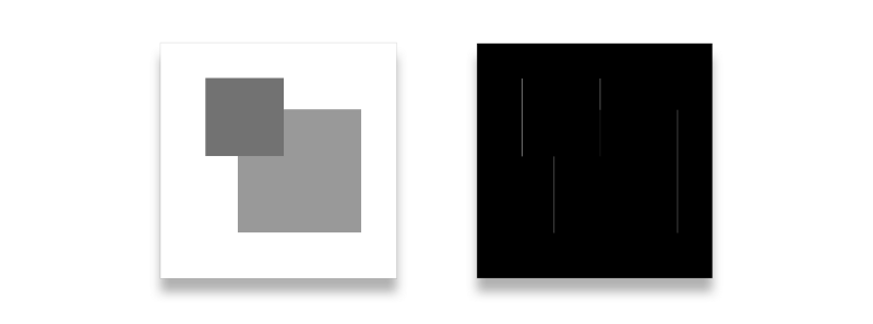
You might notice that a couple edges are missing. Specifically, the horizontal ones. In order to highlight those, we would need another kernel that looks at pixels above and below. Like this:
kernel = [
  [0  1  0]
  [0  0  0]
  [0 -1  0]
]
Also, both of these kernels won’t work well with edges of other angles or edges that are blurred. For that reason, we use many kernels (in our CapsNet implementation, we use 256 kernels). And the kernels are normally larger to allow for more wiggle room (our kernels will be 9x9).
This is what one of the kernels looked like after training the model. It’s not very obvious, but this is just a larger version of our edge detector that is more robust and only finds edges that go from bright to dark.
kernel = [
  [ 0.02 -0.01  0.01 -0.05 -0.08 -0.14 -0.16 -0.22 -0.02]
  [ 0.01  0.02  0.03  0.02  0.00 -0.06 -0.14 -0.28  0.03]
  [ 0.03  0.01  0.02  0.01  0.03  0.01 -0.11 -0.22 -0.08]
  [ 0.03 -0.01 -0.02  0.01  0.04  0.07 -0.11 -0.24 -0.05]
  [-0.01 -0.02 -0.02  0.01  0.06  0.12 -0.13 -0.31  0.04]
  [-0.05 -0.02  0.00  0.05  0.08  0.14 -0.17 -0.29  0.08]
  [-0.06  0.02  0.00  0.07  0.07  0.04 -0.18 -0.10  0.05]
  [-0.06  0.01  0.04  0.05  0.03 -0.01 -0.10 -0.07  0.00]
  [-0.04  0.00  0.04  0.05  0.02 -0.04 -0.02 -0.05  0.04]
]
Note: I’ve rounded the values because they are quite large, for example 0.01783941
Luckily, we don’t have to hand-pick this collection of kernels. That is what training does. The kernels all start off empty (or in a random state) and keep getting tweaked in the direction that makes the output closer to what we want.
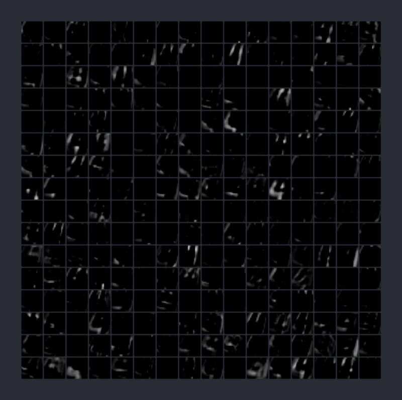
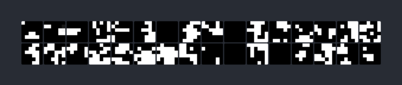
This is what the 256 kernels ended up looking like (I colored them as pixels so it’s easier to digest). The more negative the numbers, the bluer they are. 0 is green and positive is yellow:
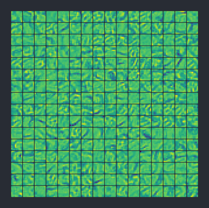
After we filter the image with all of these kernels, we end up with a fat stack of 256 output images.
Part 1b: ReLU
ReLU (formally known as Rectified Linear Unit) may sound complicated, but it’s actually quite simple. ReLU is an activation function that takes in a value. If it’s negative it becomes zero, and if it’s positive it stays the same.
In code:
x = max(0, x)And as a graph:
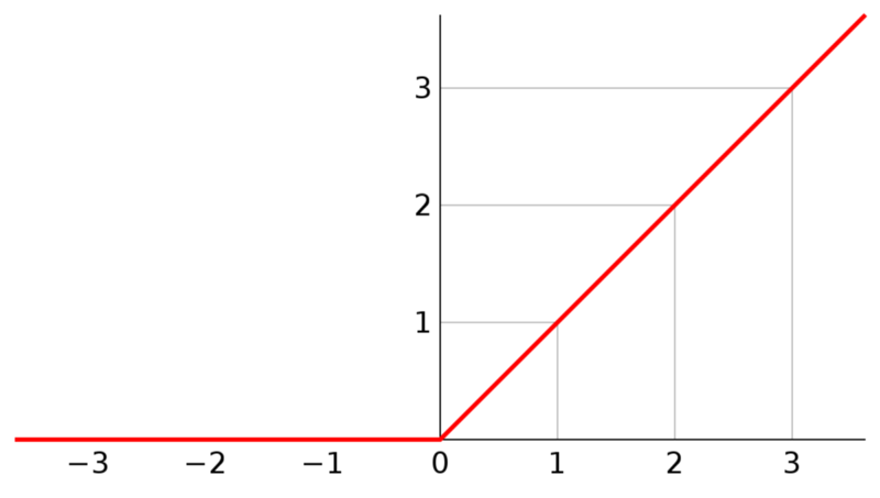
We apply this function to all of the outputs of our convolutions.
Why do we do this? If we don’t apply some sort of activation function to the output of our layers, then the entire neural net could be described as a linear function. This would mean that all this stuff we are doing is kind of pointless.
Adding a non-linearity allows us to describe all kinds of functions. There are many different types of function we could apply, but ReLU is the most popular because it’s very cheap to perform.
Here are the outputs of ReLU Conv1 layer:
Part 2a: PrimaryCaps
The PrimaryCaps layer starts off as a normal convolution layer, but this time we are convolving over the stack of 256 outputs from the previous convolutions. So instead of having a 9x9 kernel, we have a 9x9x256 kernel.
So what exactly are we looking for?
In the first layer of convolutions we were looking for simple edges and curves. Now we are looking for slightly more complex shapes from the edges we found earlier.
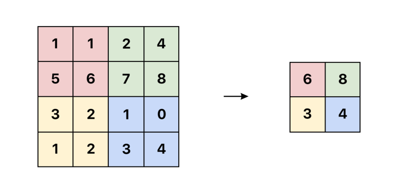
This time our “stride” is 2. That means instead of moving 1 pixel at a time, we take steps of 2. A larger stride is chosen so that we can reduce the size of our input more rapidly:
Note: The dimension of the output would normally be 12, but we divide it by 2, because of the stride. For example: ((20 — 9) + 1) / 2 = 6
We will convolve over the outputs another 256 times. So we will end up with a stack of 256 6x6 outputs.
But this time we aren’t satisfied with just some lousy plain old numbers.
We’re going to cut the stack up into 32 decks with 8 cards each deck.
We can call this deck a “capsule layer.”
Each capsule layer has 36 “capsules.”
If you’re keeping up (and are a math wiz), that means each capsule has an array of 8 values. This is what we can call a “vector.”
Here’s what I’m talking about:
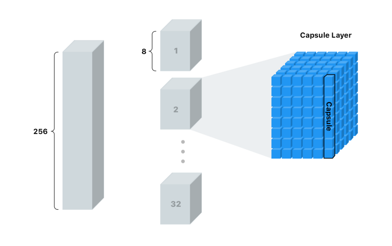
These “capsules” are our new pixel.
With a single pixel, we could only store the confidence of whether or not we found an edge in that spot. The higher the number, the higher the confidence.
With a capsule we can store 8 values per location! That gives us the opportunity to store more information than just whether or not we found a shape in that spot. But what other kinds of information would we want to store?
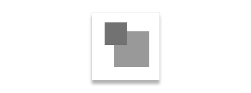
When looking at the shape below, what can you tell me about it? If you had to tell someone else how to redraw it, and they couldn’t look at it, what would you say?
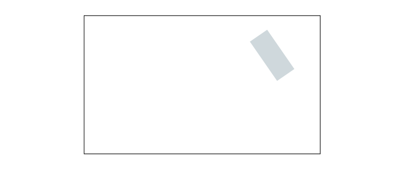
This image is extremely basic, so there are only a few details we need to describe the shape:
- Type of shape
- Position
- Rotation
- Color
- Size
We can call these “instantiation parameters.” With more complex images we will end up needing more details. They can include pose (position, size, orientation), deformation, velocity, albedo, hue, texture, and so on.
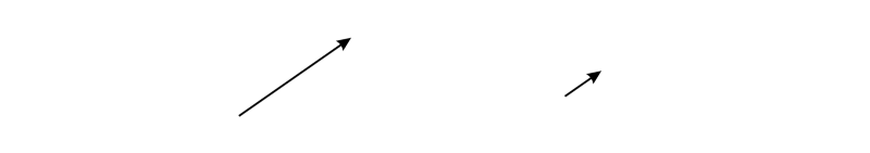
You might remember that when we made a kernel for edge detection, it only worked on a specific angle. We needed a kernel for each angle. We could get away with it when dealing with edges because there are very few ways to describe an edge. Once we get up to the level of shapes, we don’t want to have a kernel for every angle of rectangles, ovals, triangles, and so on. It would get unwieldy, and would become even worse when dealing with more complicated shapes that have 3 dimensional rotations and features like lighting.
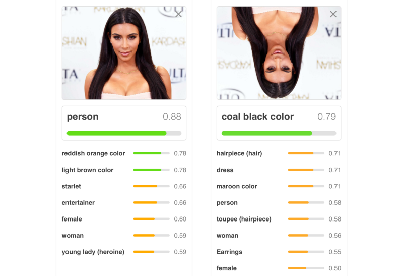
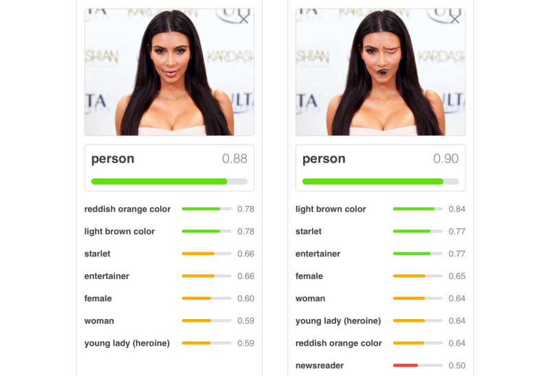
That’s one of the reasons why traditional neural nets don’t handle unseen rotations very well:
As we go from edges to shapes and from shapes to objects, it would be nice if we had more room to store this extra useful information.
Here is a simplified comparison of 2 capsule layers (one for rectangles and the other for triangles) vs 2 traditional pixel outputs:
Like a traditional 2D or 3D vector, this vector has an angle and a length. The length describes the probability, and the angle describes the instantiation parameters. In the example above, the angle actually matches the angle of the shape, but that’s not normally the case.
In reality it’s not really feasible (or at least easy) to visualize the vectors like above, because these vectors are 8 dimensional.
Since we have all this extra information in a capsule, the idea is that we should be able to recreate the image from them.
Sounds great, but how do we coax the network into actually wanting to learn these things?
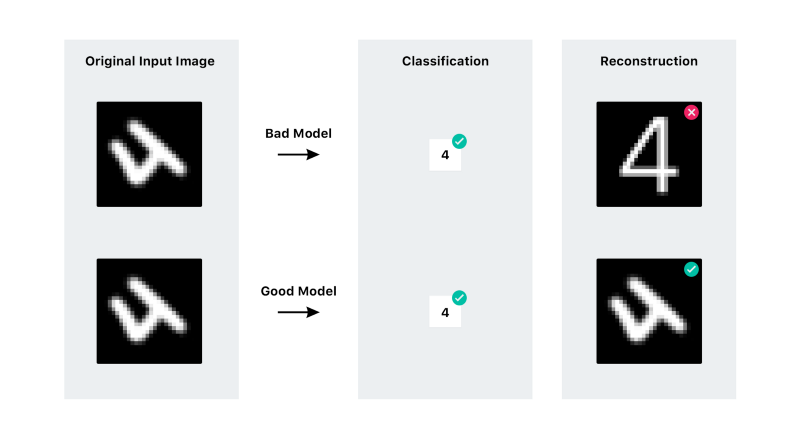
When training a traditional CNN, we only care about whether or not the model predicts the right classification. With a capsule network, we have something called a “reconstruction.” A reconstruction takes the vector we created and tries to recreate the original input image, given only this vector. We then grade the model based on how close the reconstruction matches the original image.
I will go into more detail on this in the coming sections, but here is a simple example:
Part 2b: Squashing
After we have our capsules, we are going to perform another non-linearity function on it (like ReLU), but this time the equation is a bit more involved. The function scales the values of the vector so that only the length of the vector changes, not the angle. This way we can make the vector between 0 and 1 so it’s an actual probability.
This is what lengths of the capsule vectors look like after squashing. At this point it’s almost impossible to guess what each capsule is looking for.
Part 3: Routing by Agreement
The next step is to decide what information to send to the next level. In traditional networks, we would probably do something like “max pooling.” Max pooling is a way to reduce size by only passing on the highest activated pixel in the region to the next layer.
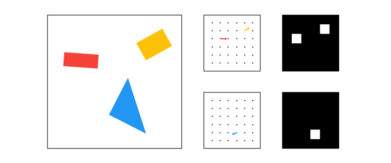
However, with capsule networks we are going to do something called routing by agreement. The best example of this is the boat and house example illustrated by Aurélien Géron in this excellent video. Each capsule tries to predict the next layer’s activations based on itself:
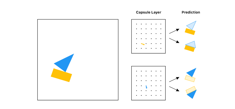
Looking at these predictions, which object would you choose to pass on to the next layer (not knowing the input)? Probably the boat, right? both the rectangle capsule and the triangle capsule agree on what the boat would look like. But they don’t agree on how the house would look, so it’s not very likely that the object is a house.
With routing by agreement, we only pass on the useful information and throw away the data that would just add noise to the results. This gives us a much smarter selection than just choosing the largest number, like in max pooling.
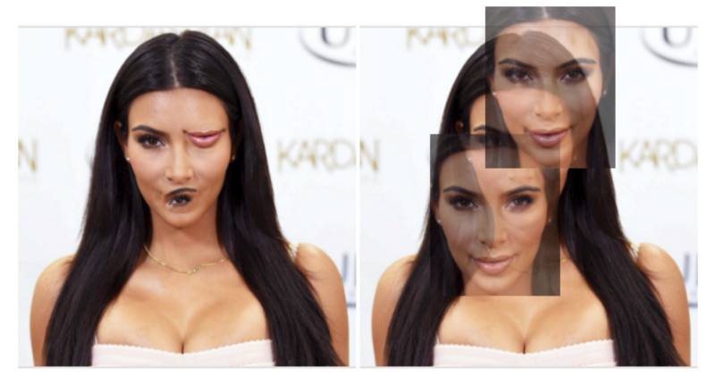
With traditional networks, misplaced features don’t faze it:
With capsule networks, the features wouldn’t agree with each other:
Hopefully, that works intuitively. However, how does the math work?
We have 10 different digit classes that we are predicting:
0, 1, 2, 3, 4, 5, 6, 7, 8, 9Note: In the boat and house example we were predicting 2 objects, but now we are predicting 10.
Unlike in the boat and the house example, the predictions aren’t actually images. Instead, we are trying to predict the vector that describes the image.
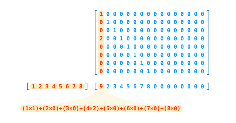
The capsule’s predictions for each class are made by multiplying it’s vector by a matrix of weights for each class that we are trying to predict.
Remember that we have 32 capsule layers, and each capsule layer has 36 capsules. That means we have a total of 1,152 capsules.
cap_1 * weight_for_0 = prediction
cap_1 * weight_for_1 = prediction
cap_1 * weight_for_2 = prediction
cap_1 * ...
cap_1 * weight_for_9 = prediction

cap_2 * weight_for_0 = prediction
cap_2 * weight_for_1 = prediction
cap_2 * weight_for_2 = prediction
cap_2 * ...
cap_2 * weight_for_9 = prediction

...

cap_1152 * weight_for_0 = prediction
cap_1152 * weight_for_1 = prediction
cap_1152 * weight_for_2 = prediction
cap_1152 * ...
cap_1152 * weight_for_9 = prediction
You will end up with a list of 11,520 predictions.
Each weight is actually a 16x8 matrix, so each prediction is a matrix multiplication between the capsule vector and this weight matrix:
As you can see, our prediction is a 16 degree vector.
Where does the 16 come from? It’s an arbitrary choice, just like 8 was for our original capsules.
But it should be noted that we want to increase the number of dimensions of our capsules the deeper we get into the network. This should make sense intuitively, because the deeper we go the more complex our features become and the more parameters we need to recreate them. For example, you will need more information to describe an entire face than just a person’s eye.
The next step is to figure out which of these 11,520 predictions agree with each other the most.
It can be difficult to visualize a solution to this when we think in terms of high dimensional vectors. For the sake of sanity, let’s start off by pretending our vectors are just points in 2 dimensional space:
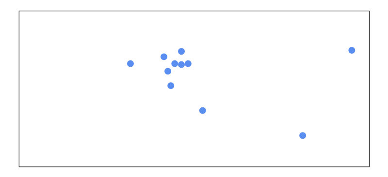
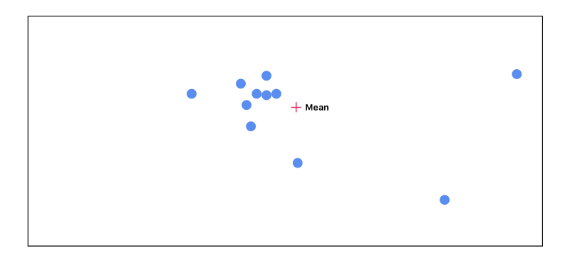
We start off by calculating the mean of all of the points. Each point starts out with equal importance:
We then can measure the distance between every point from the mean. The further the point is away from the mean, the less important that point becomes:

We then recalculate the mean, this time taking into account the point’s importance:
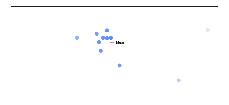
We end up going through this cycle 3 times:
As you can see, as we go through this cycle, the points that don’t agree with the others start to disappear. The highest agreeing points end up getting passed on to the next layer with the highest activations.
Part 4: DigitCaps
After agreement, we end up with ten 16 dimensional vectors, one vector for each digit. This matrix is our final prediction. The length of the vector is the confidence of the digit being found — the longer the better. The vector can also be used to generate a reconstruction of the input image.
This is what the lengths of the vectors look like with the input of 4:
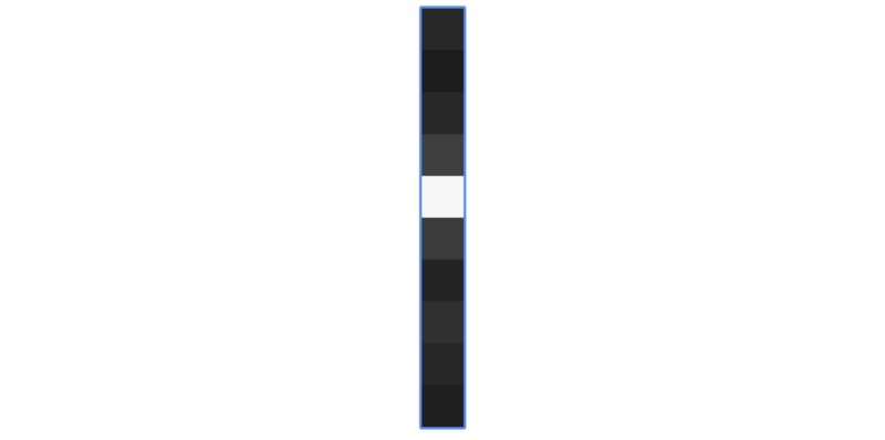
The fifth block is the brightest, which means high confidence. Remember that 0 is the first class, meaning 4 is our predicted class.
Part 5: Reconstruction
The reconstruction portion of the implementation isn’t very interesting. It’s just a few fully connected layers. But the reconstruction itself is very cool and fun to play around with.
If we reconstruct our 4 input from its vector, this is what we get:

If we manipulate the sliders (the vector), we can see how each dimension affects the 4:
I recommend cloning the visualization repo to play around with different inputs and see how the sliders affect the reconstruction:
git clone https://github.com/bourdakos1/CapsNet-Visualization.git
cd CapsNet-Visualization
pip install -r requirements.txt
Run the tool:
python run_visualization.pyThen point your browser to: http://localhost:5000
Final Thoughts
I think that the reconstructions from capsule networks are stunning. Even though the current model is only trained on simple digits, it makes my mind run with the possibilities that a matured architecture trained on a larger dataset could achieve.
I’m very curious to see how manipulating the reconstruction vectors of a more complicated image would affect it. For that reason, my next project is to get capsule networks to work with the CIFAR and smallNORB datasets.
Thanks for reading! If you have any questions, feel free to reach out at bourdakos1@gmail.com, connect with me on LinkedIn, or follow me on Medium and Twitter.
If you found this article helpful, it would mean a lot if you gave it some applause? and shared to help others find it! And feel free to leave a comment below.